
The preferred solution is always to increase the mesh resolution, to better represent the evolution of waves due to changes in bathymetric depths and/or ambient currents. But this preferred solution is not always feasible, especially when the non-physical behavior is occurring far from the region of interest.
Now this question has been addressed in a robust manner with the latest version of SWAN (starting with v41.01B) and SWAN+ADCIRC (starting with v53.00). Previous techniques are now outdated. This post will describe this new technique, and demonstrate its performance on a few test cases.
Summary of Previous Techniques
Our previous techniques to address this problem have focused on controlling where and how much the propagation velocities were allowed to evolve. These techniques had two main phases:
-
First, we tried to simply enable and disable the refraction in portions of the domain. Refraction was enabled in the region of interest, such as the coastline of the northern Gulf of Mexico during simulations of Hurricane Katrina (2005), because that region had mesh resolution that was sufficiently fine. But refraction was disabled in far-away regions, such as the Caribbean Sea during that same simulation of Katrina, because we wanted to coarsen the mesh resolution for computational efficiency. This technique led to the addition of an ADCIRC nodal attribute:
wave_refraction_in_swanThis technique was described in posts from Oct 2009 and May 2011.
-
Second, we implemented limiters on the refraction and frequency-shifting in SWAN. The limiters were based on a CFL restriction for the propagation velocities in spectral space. It was emphasized that these limiters could not eliminate the inaccuracies that were caused by insufficient resolution, but they could control the largest accuracy errors in under-resolved regions and prevent them from spreading throughout the computational domain. This technique required the addition of parameters inside the SWAN control file, specifically the line controlling its numerical properties:
NUM STOPC ... MXITNS=20 CTHETA CFL=0.25 CSIGMA CFL=0.25This technique was described in a post from Apr 2012 and an article in Ocean Modelling.
These techniques are now outdated. Users of SWAN+ADCIRC should not be using this nodal attribute, and they should not be adding these parameters inside the SWAN control file. Instead, the latest version of SWAN has been updated to address this problem in a robust manner.
Updates in SWAN 41.01B
In their patch B to v41.01, the SWAN developers implemented a few updates to how the spectral propagation velocities are computed. The turning rate is related to the bottom slope that was approximated with simple upwind schemes. Now, with this improvement, the bottom slope is replaced by the gradient of the wave number, and this gradient is approximated by means of the Green-Gauss formula. From their implementation notes:
- Calculation of turning rate improved:
- Based on derivatives of phase velocity instead of depth
- Central differences instead of upwind for computing derivatives (structured)
- Green-Gauss formula instead of upwind for computing derivatives (unstructured)
Inclusion neighboring sweeps removed
These updates will eliminate the non-physical behavior due to excessive refraction. Now, even in regions with relatively-coarse mesh resolution, the energy is not allowed to focus at a single mesh vertex and cause extreme significant wave heights. It is emphasized that these updates are blind to the user; they are used automatically in the newest version of SWAN, and there is no need to activate them with any parameter in the SWAN+ADCIRC input files.
Performance in Selected Examples
In the rest of this post, I will go back to a few test cases that we have used previously to explore this problem of excessive refraction, and then demonstrate the good performance of the new updates to the spectral propagation velocities.
Elliptic Mound in Deep Water
The first example is an idealized, elliptic mound in deep water. The bathymetric depth is 1000 m but slopes upward to 200 m at the top of the mound. The full details are given in Section 3.2.1 of our article in Ocean Modelling, including its Figure 5, modified below to include the updates.
The panels show (a) the idealized bathymetry, and (b) the coarse representation of the bathymetry in the unstructured mesh. Waves are specified at the northern boundary and propagate southward on an ambient current of 0.1 m/s. Excessive refraction is the cause of (c) significant wave heights as large as 195 m, starting at the mound and moving northwestward.
When the refraction was (d) limited with CTHETA CFL=0.5 in the SWAN control file, then the non-physical behavior was eliminated. But now, by using the latest version of SWAN and SWAN+ADCIRC, (e) the significant wave heights are not excessive, without any changes to the model input files.
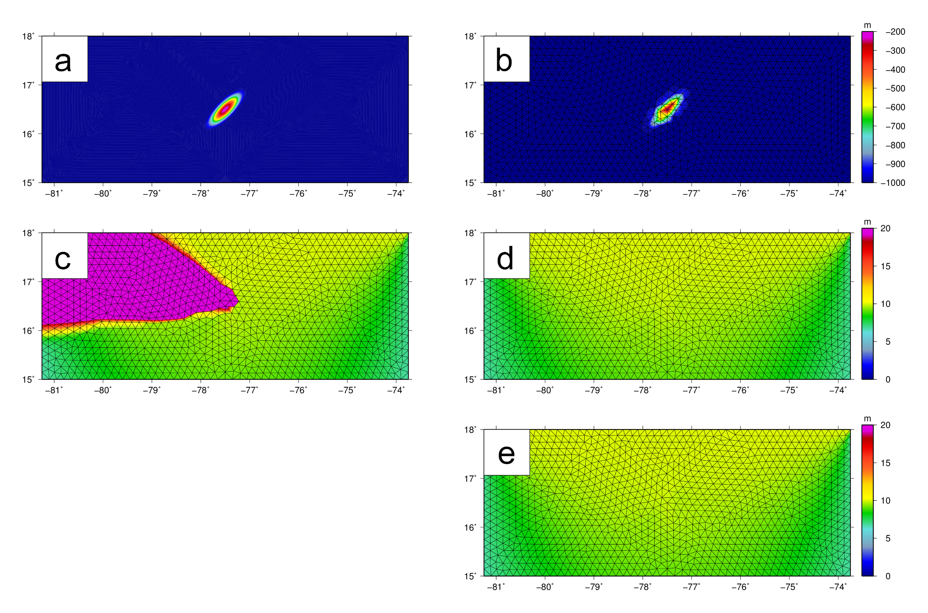
The submerged mound test domain, with panels of: bathymetry (m) from (a) idealized conditions and (b) as interpolated to the unstructured mesh, and maximum significant wave heights (m) with (c) unlimited propagation velocities, (d) the turning rate limited with CTHETA CFL=0.5, and (e) the updated treatment of the turning rate. In panel (c), the Hs range upward to 195 m.
Katrina (2005) on EC2001
The second example is Hurricane Katrina (2005) on the relatively-coarse EC2001 mesh. Mesh spacings range from 20–25 km in the Atlantic Ocean, to 15–20 km in the deeper Gulf, to 5–8 km on the continental shelves, to 1 km or less near southern Louisiana. The full details are given in Section 3.2.2 of our article in Ocean Modelling, including its Figure 9, modified below to include the updates.
The panels show the maximum significant wave heights during the simulation. Excessive refraction is the cause of (a) significant wave heights as large as 150 m, including regions far from the storm track. When the refraction was (b) limited with CTHETA CFL=0.5 in the SWAN control file, then the non-physical behavior was eliminated. But now, by using the latest version of SWAN and SWAN+ADCIRC, (c) the significant wave heights are not excessive, without any changes to the model input files.
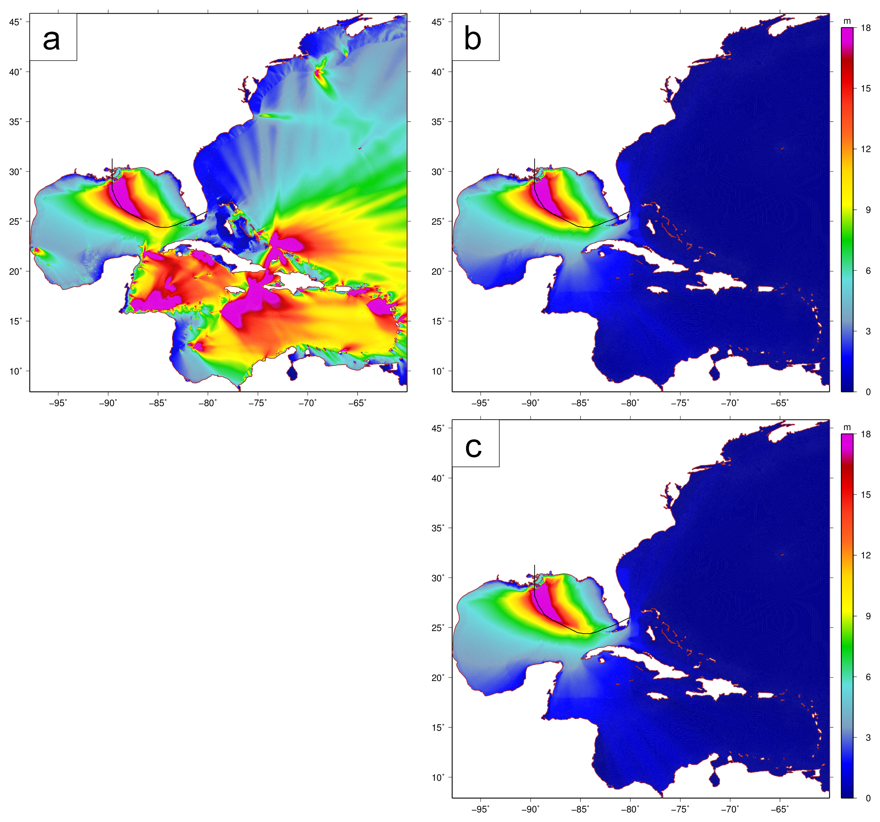
Maximum significant wave heights (m) during the Katrina hindcast on the EC2001 mesh, with panels of: (a) unlimited spectral propagation velocities, (b) the turning rate limited with CTHETA CFL=0.5, and (c) the updated treatment of the turning rate. The hurricane track is also indicated.
Coastal Ridge
The third example is an idealized coastal ridge. The depths range from 15 m in the southeast corner of the domain to 0.5 m in the floodplain to the northwest, with the ridge having a height of 1.5 m above sea level. Forcings are selected to simulate an incoming storm surge. The full details are given in Section 3.3.1 of our article in Ocean Modelling, including its Figure 11, modified below to include the updates.
The panels show (a) the idealized bathymetry, and (b) the coarse representation of the bathymetry in the unstructured mesh. Surge and waves are specified at the southern boundary, and a southerly wind is also applied. Excessive frequency shifting is the cause of (c) peak periods as large as 31.86 s, the maximum discretized period in this test.
When the refraction and frequency shifting were (d) limited with CTHETA CFL=0.25 CSIGMA CFL=0.25 in the SWAN control file, then the non-physical behavior was eliminated. But now, by using the latest version of SWAN and SWAN+ADCIRC, (e) the peak wave periods are not excessive, without any changes to the model input files.
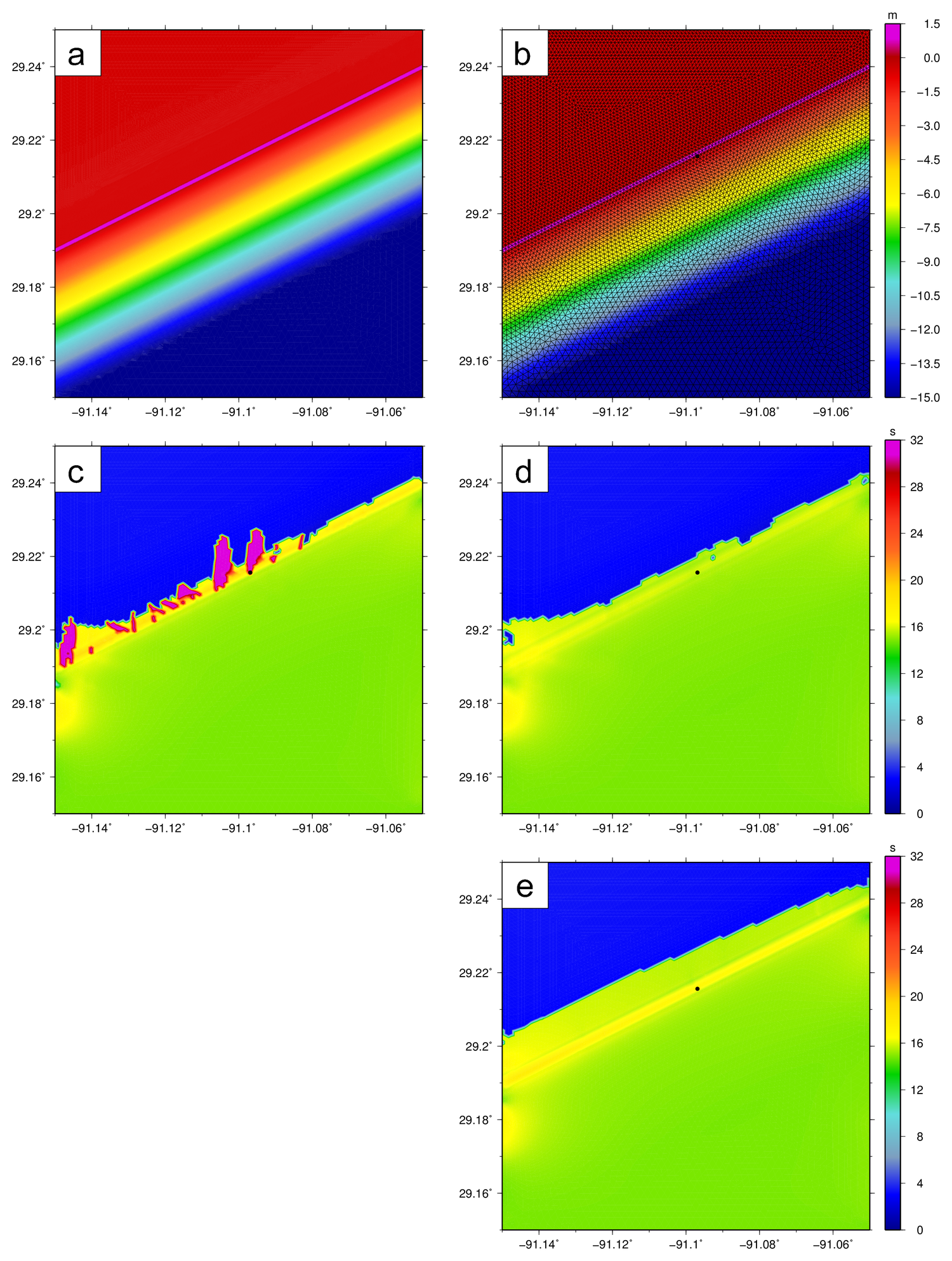
The shallow-water test domain, with panels of: bathymetry (m) from (a) idealized conditions and (b) as interpolated to the unstructured mesh, and peak wave periods (s) with (c) unlimited propagation velocities, (d) the turning rate limited with CSIGMA CFL=0.25 CTHETA CFL=0.25, and (e) the updated treatment of the spectral propagation velocities. Peak periods are shown after two days of simulation.
Hugo (1989) on SC12
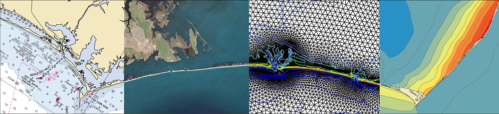
The last example is Hurricane Hugo (1989) on the SC12 mesh. The mesh spacings are 20 km or larger throughout most of the geographical domain, but they decrease significantly on the continental shelf and the coastal floodplains. The smallest mesh spacings of about 200 m are located in the region near Charleston Harbor. The full details are given in Section 3.3.2 of our article in Ocean Modelling, including its Figure 16, modified below to include the updates.
The panels show the maximum peak wave periods during the simulation. Excessive refraction and frequency shifting are the cause of (a) peak wave periods of 31.86 s, the largest discretized period. When the propagation velocities were (b) limited with CSIGMA CFL=0.25 CTHETA CFL=0.25 in the SWAN control file, then the non-physical behavior was eliminated. But now, by using the latest version of SWAN and SWAN+ADCIRC, (c) the peak wave periods are not excessive, without any changes to the model input files.
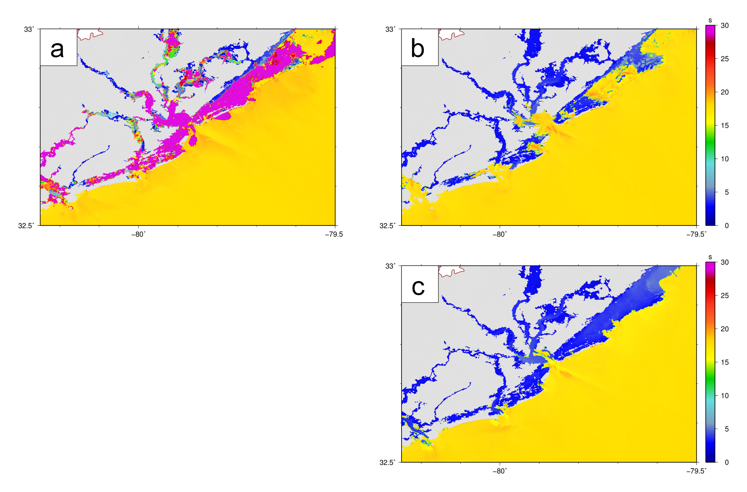
Maximum values for peak wave periods (s) near Charleston Harbor during the Hugo hindcast on the SC12 mesh. The peak periods are shown: (a) with unlimited spectral propagation velocities, (b) with both velocities limited with CSIGMA CFL=0.25 CTHETA CFL=0.25, and (c) with the updated treatment of the propagation velocities.