Controlling Errors with Limiters on Spectral Propagation Velocities

Updated 2016/07/31: This post is now outdated. SWAN has been updated to improve its treatment of the spectral propagation velocities, so these limiters are not needed. Please see this post.

Updated 2012/12/26: Added link to published manuscript.

Updated 2012/11/19: Changes to reflect our accepted submission to Ocean Modelling.

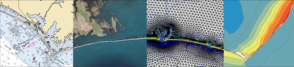
As we have gained experience with the coupling of SWAN and ADCIRC, we have noticed that SWAN can focus wave energy due to excessive refraction in regions with coarse mesh resolution. Wave energy can become focused unrealistically at a single mesh vertex, causing the wave properties to become non-physical. In deep water, the significant wave heights can become 150m or larger. In shallow water, the peak wave periods can become 30s or larger, as the energy is pushed into the lowest-discretized frequency bin.

We have developed a few work-around solutions to this problem (Part 1 and Part 2). These solutions have enabled the wave refraction process in the region of interest, and disabled it elsewhere in the computational domain. For example, by enabling selectively the refraction in the northern Gulf of Mexico, we can obtain the following hindcast of the significant wave heights during Hurricane Gustav (2008).

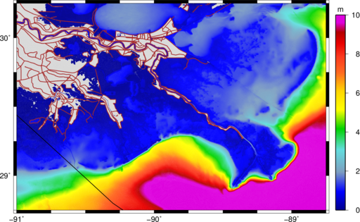
Maximum significant wave heights (m) during Gustav (2008).

However, a more robust solution would be the limiting of the spectral propagation velocities, especially the directional turning rate, based on the Courant-Friedrichs-Lewy (CFL) condition. We have implemented recently these limiters in SWAN+ADCIRC. On this page, the limiters are introduced and tested on idealized and realistic applications.

It should be noted that these limiters are not a replacement for increased mesh resolution. The SWAN solution will always be better when the mesh is improved to represent the bathymetric gradients in the region of interest. However, when it is not feasible to increase the mesh resolution, then these limiters can control the largest SWAN errors without affecting the solution elsewhere.

If you would like to receive more information about these limiters, then please see our manuscript from Ocean Modelling.

Theory:

The propagation velocities in spectral space are given by:

$\begin{equation*} \begin{aligned} c_\sigma = \frac{| \vec{k} | \sigma}{\sinh (2 | \vec{k} | H )} &\biggl( \frac{\partial H}{\partial t} + \frac{u_\lambda}{R \cos \varphi} \frac{\partial H}{\partial \lambda} + \frac{u_\varphi}{R} \frac{\partial H}{\partial \varphi} \biggr) \\ - \frac{c_g | \vec{k} |}{R} &\biggl( \frac{1}{\cos \varphi} \frac{\partial u_\lambda}{\partial \lambda} \cos^2 \theta + \frac{\partial u_\lambda}{\partial \varphi} \cos \theta \sin \theta \\ &+ \frac{1}{\cos \varphi} \frac{\partial u_\varphi}{\partial \lambda} \sin \theta \cos \theta + \frac{\partial u_\varphi}{\partial \varphi} \sin^2 \theta \biggr) \end{aligned} \end{equation*}$

and:

$\begin{equation*} \begin{aligned} c_\theta = \frac{\sigma}{R \sinh (2 | \vec{k} | H )} &\biggl( \frac{1}{\cos \varphi} \frac{\partial H}{\partial \lambda} \sin \theta - \frac{\partial H}{\partial \varphi} \cos \theta \biggr) \\ + \frac{1}{R} &\biggl( \frac{1}{\cos \varphi} \frac{\partial u_\lambda}{\partial \lambda} \cos \theta \sin \theta - \frac{\partial u_\lambda}{\partial \varphi} \cos^2 \theta \\ &+ \frac{1}{\cos \varphi} \frac{\partial u_\varphi}{\partial \lambda} \sin^2 \theta - \frac{\partial u_\varphi}{\partial \varphi} \sin \theta \cos \theta \biggr) \\ &- \biggl( \frac{c_\lambda \cos \theta + c_\varphi \sin \theta}{R} \biggr) \cos \theta \tan \varphi \end{aligned} \end{equation*}$

where $\vec{k} = (k_\lambda, k_\varphi) = (| \vec{k} | \cos \theta, | \vec{k} | \sin \theta)$ is the wave number vector, $H = h + \zeta$ is the total water depth, $h$ is the bathymetric depth measured downward from the mean water level, $\zeta$ is the water surface deviation from the mean, $c_g$ is the group velocity, $\vec{u} = (u_\lambda,u_\varphi)$ are the ambient currents, and $R$ is the radius of the Earth. Diffraction is handled separately. The quantities $\zeta$ and $\vec{u}$ are provided via the tight coupling with ADCIRC, as described below.

Because the solution method is implicit, the propagation velocities are not limited by the CFL condition for stability. However, we will show that the velocities should be limited for accuracy reasons. The CFL conditions can be expressed as:

(1) $\begin{equation*} \mathbb{C}_\theta = \frac{c_\theta \Delta t}{\Delta \theta} < \alpha_\theta \end{equation*}$

and:

(2) $\begin{equation*} \mathbb{C}_\sigma = \frac{c_\sigma \Delta t}{\Delta \sigma} < \alpha_\sigma \end{equation*}$

where $\mathbb{C}_\theta$ and $\mathbb{C}_\sigma$ are the CFL conditions for the propagation velocities $c_\theta$ and $c_\sigma$ , respectively. The coefficients $\alpha_\theta$ and $\alpha_\sigma$ will be selected to prevent the excessive directional turning and frequency shifting that can lead to non-physical behavior. However, in practice, the SWAN time step $\Delta t$ is too large and thus too restrictive in Equations 1–2. By using the CFL condition in geographic space, these equations can be simplified to obtain the following expressions for the turning rate:

(3) $\begin{equation*} c_\theta < \alpha_\theta \Delta \theta \biggl( \frac{c_\lambda}{\Delta \lambda} + \frac{c_\varphi}{\Delta \varphi} \biggr) \end{equation*}$

and the frequency shifting:

(4) $\begin{equation*} c_\sigma < \alpha_\sigma \Delta \sigma \biggl( \frac{c_\lambda}{\Delta \lambda} + \frac{c_\varphi}{\Delta \varphi} \biggr) \end{equation*}$

The proper selection of $\alpha_\theta$ and $\alpha_\sigma$ in Equations 3–4 will limit the spectral propagation velocities, and thus prevent wave energy from turning excessively during a single time step. The results presented herein will support a selection of $\alpha_\theta$ and $\alpha_\sigma$ in the range of 0.25-0.5, but the user may specify any coefficients at run-time.

Implementation:

The limiters are controlled with commands in the SWAN control file (which is typically called fort.26 in the SWAN+ADCIRC coupling). Specifically, commands are added to the end of the NUMERICS line. For example, we typically use the line:

NUM STOPC DABS=0.005 DREL=0.01 CURVAT=0.005 NPNTS=95 NONSTAT MXITNS=20

which represents the default convergence criteria for unstructured meshes, except that we relax the requirement on the percentage of vertices that must show convergence, so that we have NPNTS=95.

The limiter on $c_\theta$ is set by adding to the end:

NUM STOPC ... NONSTAT MXITNS=20 CTHETA CFL=0.5

or you can set both limiters by adding:

NUM STOPC ... NONSTAT MXITNS=20 CSIGMA CFL=0.25 CTHETA CFL=0.25

Note that the order is important. If you are setting the limiters for both $c_\sigma$ and $c_\theta$ , then they need to appear in that order on the NUMERICS line. SWAN will limit the spectral propagation velocities to prevent excessive refraction and/or frequency shifting.

Idealized Test Case:

Coastal regions often contain complex geometries, steep bathymetric gradients, small-scale islands and channels, etc., which require high levels of resolution. An idealized example is shown in Figure 1a. This test case is a rectangular $0.1^{\circ}$ domain that reproduces the shoaling of waves over a coastal ridge, as in the hindcast of Gustav (2008) in the section below. The depths range from 15m in the southeast corner of the domain to 0.5m in the floodplain to the northwest, with the ridge having a height of 1.5m above sea level.

Forcings are selected to simulate an incoming storm surge. In ADCIRC, the water levels are raised by 2m and a current of 2 m/s is specified at the south boundary. In SWAN, an incoming wave is specified at the south boundary with a JONSWAP spectrum characterized by a peak enhancement parameter $\gamma = 3.3$ , a significant height $H_s = 6$ m, a peak period $T_p = 15$ s, a mean direction of $90^{\circ}$ (northward), and a directional standard deviation of 30 $^{\circ}$ . A constant, northward wind speed of 30 m/s is applied to both SWAN and ADCIRC.

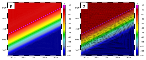
Figure 1: The shallow-water test domain, with panels of: (a) idealized bathymetry (m), and (b) bathymetry (m) interpolated to the unstructured mesh.

The domain is discretized on a relatively coarse mesh (Figure 1b), with element sizes that vary from about 200m offshore to about 100m at the ridge and inland. A line of vertices is placed along the top of the ridge, but otherwise the finite elements are generated automatically by the Surface-water Modeling Solution (SMS) software.

This mesh contains 15,449 geographic elements. Bathymetry is interpolated linearly from the idealized conditions. The spectral domain is discretized with 30 frequency bins that are distributed logarithmically from 0.031-0.55Hz, as well as constant directional bins with $\Delta \theta = 1^{\circ}$ . (Note that this directional discretization is small in comparison to studies on real domains, which typically use bins of $\Delta \theta = 5-10^{\circ}$ , but this discretization was necessary to replicate the non-physical behavior on this relatively simple test domain.)

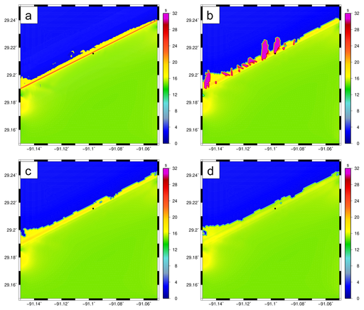
Figure 2: Peak periods (s) after two days of simulation on the shallow-water test domain, with panels of: (a) ‘true’ solution on an over-resolved mesh, (b) unlimited propagation velocities, (c) turning rate limited with a CFL condition of 0.25, and (d) peak wave periods (s) both velocities limited with CFL conditions of 0.25. The black dot in each sub-figure indicates the geographic location where variance densities are shown in Figure 3.

A “true” solution was developed by refining this mesh until the solution did not change. This fine mesh contains 3,064,699 geographic elements, and the resolution along the ridge is decreased to about 6m. When the incoming waves encounter the shallow bathymetry and ultimately move over the ridge, they shoal and experience an increase in their peak periods.

This behavior is captured on the fine mesh (Figure 2a), where the peak periods increase to about 24s at the ridge. However, on the original mesh (Figure 2b), the peak periods increase to only about 17-18s along most of the ridge, and, at a few vertices along the ridge, excessive refraction causes the the peak periods to increase to 32s.

These non-physical peak periods are the result of the turning and shifting of wave energy into smaller discretized frequencies. The variance densities at a geographic vertex near the coastal ridge are shown in Figure 3. On the fine mesh, the variance densities are smooth and have their largest values at a frequency of about 0.0625Hz, corresponding to a peak period at this location of about 16s as the waves begin to shoal over the coastal ridge. Most of this behavior is replicated on the original mesh (Figure 3b), although the solution is not smooth, and an extraneous peak is located eastward and at a smaller frequency. The variance densities are three orders of magnitude larger at this location.

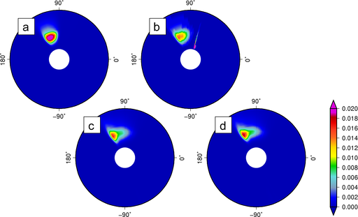
Figure 3: Variance densities in spectral space at the geographic vertex near the coastal ridge, with panels corresponding to: (a) ‘true’ solution on a fine mesh with extra resolution in geographic space, (b) unlimited propagation velocities on the coarse mesh, (c) the turning rate limited with a CFL condition of 0.25, and (d) both velocities limited with CFL conditions of 0.25.

When the refraction and frequency shifting are limited with $\alpha_\theta = \alpha_\sigma = 0.25$ (Figures 3c-d), the extraneous peak is removed and the computed solution is smooth and reasonable, although the variance densities are asymmetric and centered at a different frequency in comparison to the solution on the fine mesh. This behavior is evident in the peak periods in Figures 2c-d, as their values of 16-18s are smaller than the “true” solution with shoaling of peak periods up to 24s. The limiters improve the computed solution by preventing excessive refraction and frequency shifting, but they are not a substitute for increased mesh resolution in geographic space.

A benefit of this test case is that it can be refined in geographic space to provide a “true” solution. The coarse solution is compared to the unlimited solution on an over-resolved mesh with bathymetry re-interpolated from the idealized conditions. To obtain guidance on the proper selection of $\alpha_\theta$ , the limiter was varied over several orders of magnitude, and global error norms were computed relative to the true solution on the over-resolved mesh. The root-mean-square ( $\textit{RMS}$ ) error was computed as:

$\begin{equation*} RMS = \sqrt{ \frac{1}{N_P} \sum_{i=1}^{N_p} ( P_{i,coarse} - P_{i,fine} )^2 } \end{equation*}$

and the $L_\infty$ norm was computed as:

$\begin{equation*} L_\infty = \max ( P_{i,coarse} - P_{i,fine} ) \end{equation*}$

where $N_P$ is the number of geographic vertices on the coarse mesh, and $P_i$ are the integrated wave parameters (either $H_s$ or $T_p$ ) on the coarse and fine meshes.

The depth-limited breaking prevents the significant wave heights from growing to the same large values as in the previous section, and thus the $RMS$ and $L_\infty$ errors are reasonable (Figure 4). However, when the velocities are unlimited, the peak periods have an $RMS$ error of about 2s and an $L_\infty$ error of about 16s. When the limiters are enabled so that $\alpha_\theta \le 5$ , the solution improves so that the peak periods have an $RMS$ error of about 0.7s and an $L_\infty$ error of about 7s. This maximum error is still large, and it reflects the difference in the shoaling over the coastal ridge between the coarse and fine meshes. When the frequency shifting is also limited with $\alpha_\sigma$ , the errors are nearly identical for this test case.

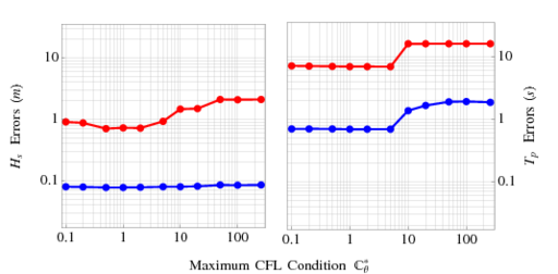
Figure 4: RMS (blue) and Linf (red) errors on the shallow-water test domain, with panels of significant wave heights (left) and peak wave periods (right). When the turning rate is unlimited, the modified CFL condition is 296 at the top of the ridge. The errors are nearly identical when both velocities are limited (not shown).

The first choice for improving the accuracy of the computed solution should always be to increase the mesh resolution. However, as this test case demonstrates, that choice is not always economical. In order to remove completely the non-physical behavior caused by the excessive wave refraction, the original mesh must be refined so that the element sizes are about 6m on the coastal ridge. This refinement increases the overall size of the mesh by a factor of about 200, and the ADCIRC time step must be reduced by a factor of 50 to maintain stability. These refinements have obvious implications on computational cost. If the available computing re- sources do not support this level of refinement, then the spectral propagation velocity limiters can control economically the largest errors.

Gustav (2008) in the Marshes of Louisiana:

Gustav tracked over Cuba, moved across the Gulf and made landfall in southern Louisiana as a strong Category 1 storm. Although Gustav passed west of the delta and farther from the city of New Orleans than did Katrina, its large size allowed it to push waves and surge onto the Louisiana-Mississippi continental shelf, where they were dissipated within the marshes and against the levee protection system. There was no flooding of the city, but there were reports of waves overtopping the seawalls.

The recent landfalling storms in the Gulf of Mexico are described by a wealth of measurement data, including observations of wind-sea wave parameters within the marshes of Louisiana. The Coastal Hydraulics Laboratory (CHL) of the U.S. Army Engineer Research and Development Center (USA-ERDC) deployed pressure gages in six locations within the Biloxi and Terrebonne marshes prior to the landfall of Gustav . The gages were sampled hourly at 2Hz. It should be noted that the spectral analysis resulted in peak periods near the high-frequency cutoff, which can result in amplification of noise and either over- or under-estimation of wave height and under-estimation of wave period. However, these gages provide a valuable description of the evolution of the wind-sea waves generated as Gustav progressed through southern Louisiana, and they offer an excellent test for the propagation velocity limiters in the nearshore. Previous studies using SWAN+ADCIRC utilized hundreds of measured time series and high-water marks to describe the evolution and validate the simulation of waves and surge from deep water to the coastal floodplains.

The focus herein is the effect of the limiters on the SWAN solution at the six CHL gage locations within the marshes. The Gustav hindcast is simulated on the Southern Louisiana (SL16) unstructured mesh. This mesh has resolution within the Gulf of Mexico of 4-6km, along the continental shelf of 1km or less, within southern Louisiana of 200m or less, and within the small-scale channels of 20-50m. The mesh provides high levels of resolution throughout the coastal floodplains, including the Biloxi and Terrebonne marshes where the CHL gages are located. The SL16 mesh contains 9,945,623 triangular elements. This Gustav simulation utilizes an 18-day tidal spin-up, and then the wind fields are applied for a 10.5-day simulation of SWAN+ADCIRC. The spectral space in SWAN is discretized with 36 directional bins with spacing $10^{\circ}$ and 40 frequency bins with logarithmic spacing over the range 0.031-1.42Hz.

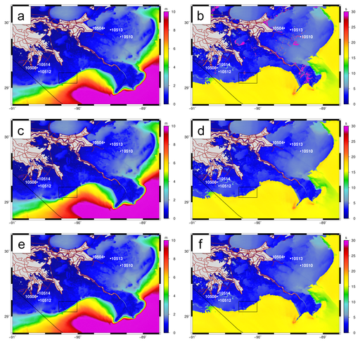
Figure 5: Maximum values for significant wave heights (m) and peak wave periods (s) in southeastern Louisiana during the Gustav hindcast on the SL16 mesh. Significant heights are shown in the left column in panels (a), (c) and (e); and peak periods are shown in the right column in panels (b), (d) and (f). The top row of panels (a) and (b) are results with unlimited spectral propagation velocities; the middle row of panels (c) and (d) are results with the turning rate limited with a CFL condition of 0.25; and the bottom row of panels (e) and (f) are results with both velocities limited with CFL conditions of 0.25. In each panel, the black box indicates the extents of the zoom shown in Figure 6.

Gustav generated waves with significant heights of 15m in the deeper Gulf, and these waves dissipated as they moved onto the continental shelf. The SWAN+ADCIRC simulation produces waves with significant heights that are entirely physical in southeastern Louisiana (Figure 5a), partly because the waves are depth-limited within the nearshore, and thus they are not allowed to become non-physical. However, the peak periods (Figure 5b) have maximum values of 31.86s, the upper limit of the discretized frequency spectrum, in many inland water bodies and the distributaries of the Mississippi River. These peak periods are non-physical.

When the turning rate is limited with $\alpha_\theta = 0.25$ (Figures 5c-d), the significant heights are not affected, but the peak periods are improved. In deeper water, the peak periods have maximum values of 16-18s that correspond to the swell waves as they approach the coast. In the nearshore, the peak periods have maximum values of 3-6s that correspond to the locally-generated wind-sea within the marshes. The non-physical peak periods of 31.86s have disappeared throughout most of the region.

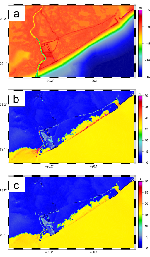
Figure 6: Details of the Gustav hindcast near Port Fourchon, Louisiana, with panels of: (a) bathymetry (m) in the SL16 mesh; (b) maximum peak wave periods (s) with the turning rate limited with a CFL condition of 0.25; and (c) maximum peak wave periods (s) with both velocities limited with a CFL condition of 0.25.

The exceptions are localized along the coastline. Figure 6 shows the maximum peak wave periods between Grand Isle and Port Fourchon. In this region, the mesh spacings range from about 200m on the continental shelf to about 100m inland. When only the turning rate is limited with $\alpha_\theta = 0.25$ (Figure 6b), the peak periods become non-physical at a line of mesh vertices along the coastline, as the swell waves approach and overtop the coastal ridge. When the frequency shifting is also limited with $\alpha_\sigma = 0.25$ (Figure 6c), there is still shoaling over the coastal ridge, but now the maximum peak periods of 20-21s are contained within the discretized frequency spectrum, and not too much longer than the 15-16s peak periods of the swell waves on the narrow continental shelf.

At the CHL gages, the time series are also improved. When the velocities are unlimited (red lines in Figure 7), the computed peak periods at gage 10510 are the non-physical 31.86s during the days leading to landfall, and gage 10504 also shows peak periods that are too large during this timeframe. This non-physical behavior is removed when the velocities are limited with $\alpha_\theta = \alpha_\sigma = 0.25$ . The significant heights match well to the maximum values of 0.5-1m, depending on the gage, and the peak periods also match the 3-6s waves associated with the wind-sea over the marshes.

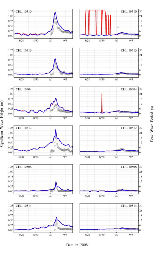
Figure 7: Time series for significant wave heights (m) and peak wave periods (s) at the CHL gages during Gustav. Gray circles are the observations, solid red lines are the results with unlimited spectral propagation velocities, and solid blue lines are the results with the velocities limited with a CFL condition of 0.25. The gage locations are shown in Figure 5.

Conclusions:

This work proposes and evaluates CFL-based limiters for the spectral propagation velocities in the unstructured-mesh version of SWAN. These limiters prevent the excessive refraction that can occur on coarse meshes. In deep water, excessive directional turning can focus energy at a single mesh vertex and create significant wave heights of 150m or larger, but the limiter on the turning rate was shown to prevent this behavior. And in the nearshore, excessive directional turning and frequency shifting can push wave energy to the smallest discretized frequency bin and create peak wave periods of 30s or larger, but the limiters on both velocities were shown to prevent this behavior.

These limiters are not a replacement for mesh refinement, which is the preferred method for reducing and eliminating numerical errors. However, when the available computing resources do not allow for the highest levels of mesh resolution, the limiters can control the largest accuracy errors without deteriorating the overall solution.