
Updated 2012/04/12: This is an old page. It persists on this site for posterity, but the information presented below is no longer up-to-date. When you are done here, then please click forward to this page, which describes how to control refraction errors with limiters on the spectral propagation velocities.
In a previous page on wave refraction, it was shown that mesh resolution plays an important role in how SWAN handles this physical process. If the mesh is resolved coarsely, then SWAN can refract too much energy, resulting in spikes in the wave solution. In our hurricane applications, we have observed spikes in the significant wave heights of 75m or larger, focused at only a few vertices, because the mesh in those regions does not resolve properly a shallow feature.
To address this problem, we added wave refraction as an attribute to the ADCIRC fort.13 file, so that it can be varied spatially. The user can enable refraction in regions with the necessary level of mesh resolution, and disable refraction in regions that are resolved coarsely. We enabled wave refraction along the northern Gulf coastline and within southern Louisiana, and we no longer saw the spikes in the significant wave heights in the regions offshore.
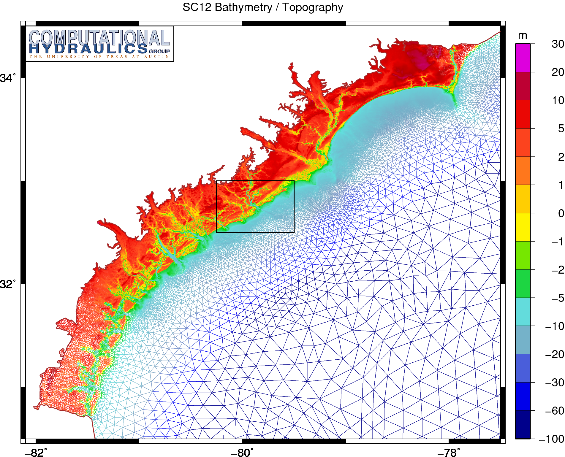
Bathymetry and topography (m) on the SC12 unstructured mesh.
Peak Periods TPS in South Carolina
However, we have learned recently that wave refraction on coarse meshes can be problematic in other ways besides creating spikes in the significant wave heights. For example, in very shallow regions, the dissipation of bottom friction and breaking would limit the significant wave heights to reasonable values, even if wave refraction was a problem. There would not be any spikes in the significant wave heights. But the focusing of wave energy would be apparent in other ways that are more subtle, such as the existence of peak periods with the maximum possible values.
On this page, we examine an instance of this problem with wave refraction on coase meshes. As a specific example, we consider a mesh that was developed for a flood inundation study along the coastline of South Carolina. It should be noted that, although this example mesh does exhibit these problems with wave refraction, the problems are also evident on other meshes and other applications. For example, we have seen similarly problematic peak periods in our hurricane applications in southern Louisiana. As we have noted previously, any wave model would face this problem of how to handle refraction on unstructured meshes.
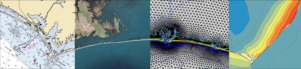
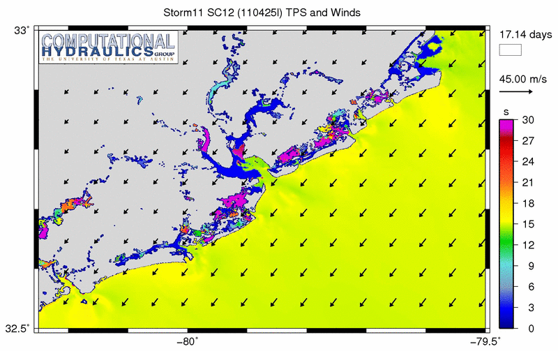
The image above shows a mesh that is being used to examine flooding risk along the South Carolina coastline. Although the image above shows only the coastline, the mesh offers coverage of the entire Western North Atlantic Ocean, Caribbean Sea, and Gulf of Mexico. The majority of its resolution is focused near South Carolina. Note how quickly the resolution varies from deep water to the coastline; the triangular elements in the lower right of the figure have sizes of 10-20km. The mesh has a total of 542,809 vertices and 1,073,925 triangular elements.
The black rectangle indicates the region near Charleston, which is depicted in the following image:
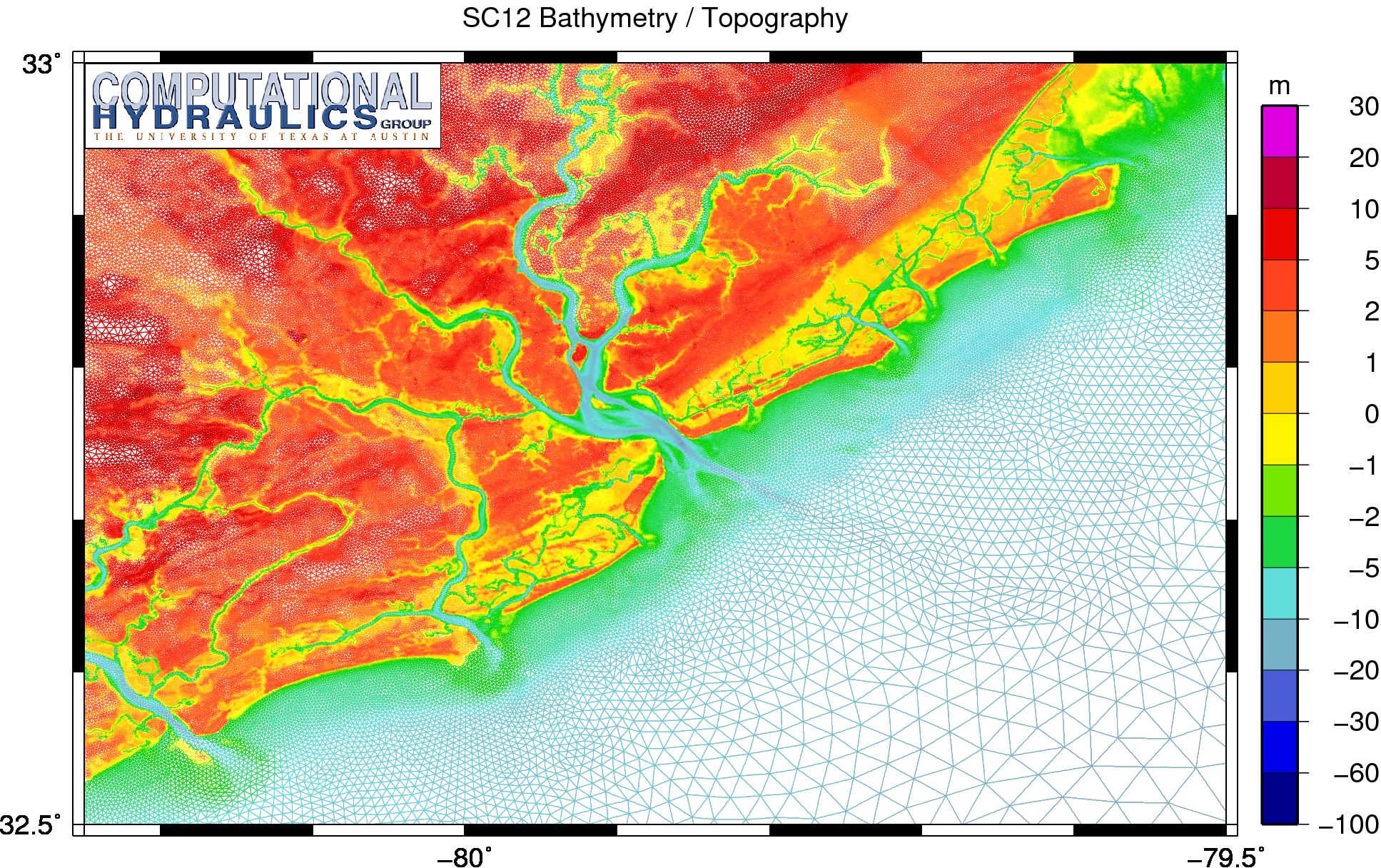
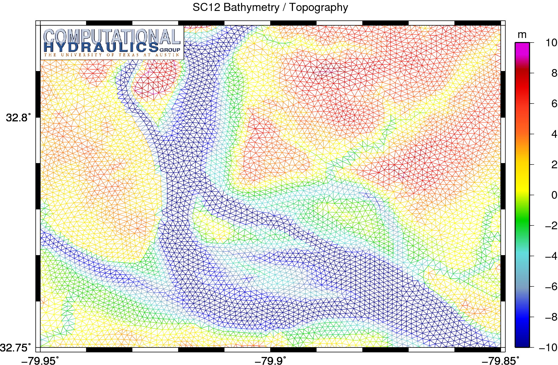
Bathymetry and topography (m) on the SC12 mesh in the region near Charleston, South Carolina.
At this zoom level, it is easier to see the intricacies of the Charleston Harbor and the rivers that connect to it. These features are resolved in the mesh with a fair level of resolution, as shown in the following image:
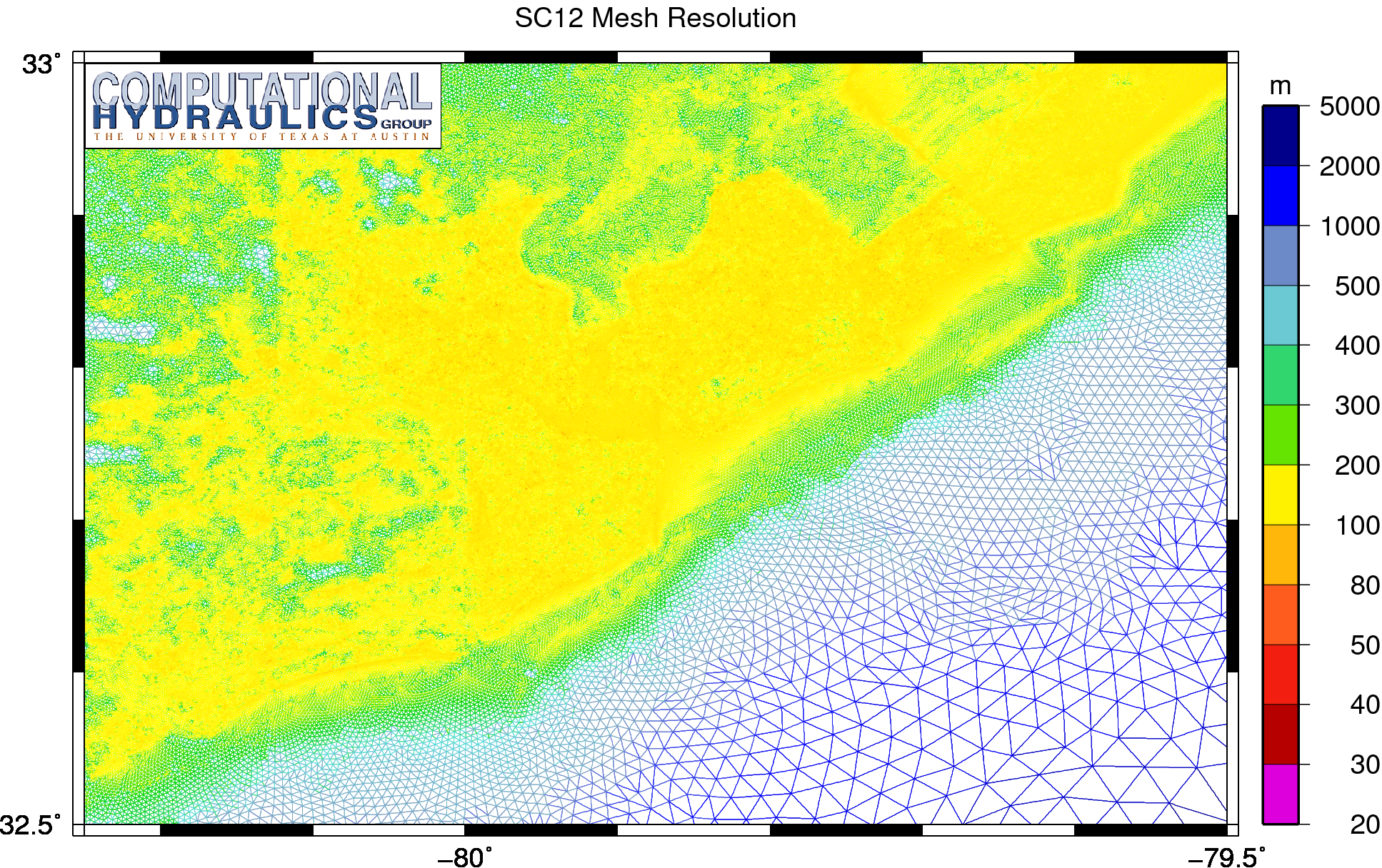
Unstructured mesh resolution (m) on the SC12 mesh in the region near Charleston, South Carolina.
This study required a delicate balance between accuracy and efficiency. The statistical analysis of flooding risk is based on a relatively large number of simulations. The storm characteristics must be varied in a manner that is significant statistically, and thus the storms will have varying intensities and landfall locations. This large set of simulations can require a significant amount of computational resources. Thus, the mesh must be as small and efficient as possible, while still providing coverage of the physical features of interest.
As shown above, the resulting mesh offers resolution down to about 100m in the harbor and channels, but the resolution coarsens quickly along the coastline and outward to the continental shelf. In the lower right of the image, the mesh sizes are about 2-3km. Thus the mesh sizes are varying over an order of magnitude from the continental shelf into the inland harbor and channels.
It is interesting to see how this mesh responds to some of the synthetic storms. The animation below shows an example of the peak wave periods (using the TPS output from SWAN) as one storm moves through the region:
Peak wave periods (s) during a synthetic storm.
This is a tricky problem, because we are looking at the back side of the storm, where the winds are blowing offshore. In many parts of this region, the wave energy spectrum is dual-peaked. One peak corresponds to the longer swell waves that were generated by the storm offshore; these long waves have periods of 15-18s and are moving toward shore. The other peak corresponds to the wind-sea; these shorter local waves have periods of 6-9s and are moving offshore with the wind.
We use the TPS peak periods that are output by SWAN. As noted in its online User Manual, “[t]his value is obtained as the maximum of a parabolic fitting through the highest bin and two bins on either side the highest one of the discrete wave spectrum.” In other words, SWAN finds the frequency bin with the highest energy, and then it fits a parabola through the energy in that bin and its neighbors.
As we will show below, this definition of peak period (and any other definition) loses its meaning when the spectrum is dual-peaked. The “peak” period can oscillate, depending on which peak is larger at the time. We can see this in the animation. Offshore, the peak periods transition from long to short as the wind-sea begins to dominate the spectrum.
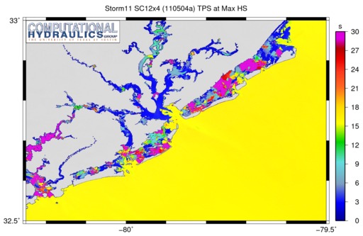
However, in the animation above, the largest peak periods are problematic for other reasons. Behind the barrier islands and within the harbor and channels, there are a lot of purple regions, indicating peak periods of 30s or longer. The bathymetry is too shallow in these regions to support waves with these long periods. This problematic behavior is more evident if we examine a plot of the peak periods corresponding to the time of the maximum significant wave heights:
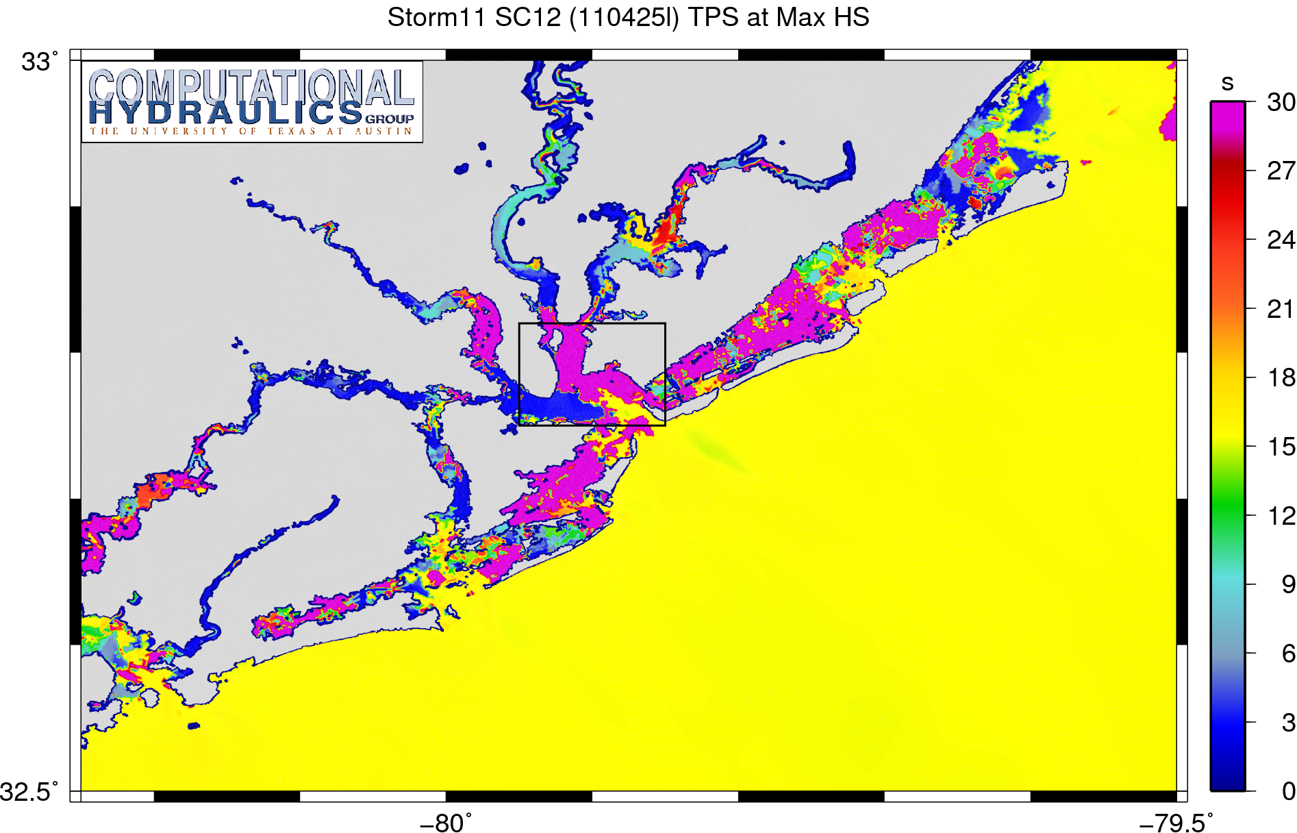
Peak wave periods (s) corresponding to the maximum significant wave height (m) during a synthetic storm.
(Note that these are not necessarily the maximum peak periods, but rather they are the peak periods corresponding to the time of the maximum significant wave height at each of the mesh vertices.)
Most of the inland harbors and channels experience peak periods larger than 30s during the simulation. Again, this behavior is unrealistic physically, because the bathymetry is too shallow in these regions to support waves with periods of this length. There must be a numerical cause for this problem.
To examine further, let’s zoom into the region indicated by the black rectangle in the previous figure. This zoom region contains part of the Charleston Harbor between the USS Yorktown State Park and the city itself. As shown above, this part of the mesh has the highest resolution of about 100m.
Bathymetry and topography (m) on the SC12 mesh near the USS Yorktown State Park.
The USS Yorktown State Park is located near the center of this zoom, in the red triangular region of relatively higher land to the northeast of the harbor. Downtown Charleston is located on the peninsula to the left in the zoom. The harbor has several deep shipping channels, separated by an uninhabited island. Fort Sumter is located to the southeast, just outside of the zoom.
The problematic spikes in the peak periods are more evident at this zoom level:
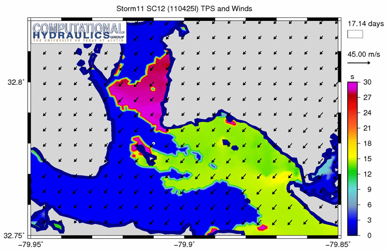
Peak wave periods (s) near the USS Yorktown State park during a synthetic storm.
It is interesting to note that some of the offshore swell does propagate to this location within the harbor. This animation shows the last stages of that propagation, just as the local wind-sea begins to dominate the spectrum. As the animation progresses, most of the peak periods become very small, on the order of 3-6s.
However, the spikes in the peak periods are very evident in this animation, especially near the USS Yorktown State Park. We see purple regions indicating peak periods of 30s or longer for most of the simulation. Of the inland regions within this mesh, this region contains some of the deepest bathymetry, and thus it can support larger, longer waves than the rest of the mesh. But these 30s waves are still unrealistic physically.
It is also interesting to note that, although the spurious peak periods are often present throughout the bay, they always start at the edges. This behavior is understandable; the bathymetry would change rapidly at the edge of the bay, as it transitions to the topography at the wet/dry interface. If this transition is not resolved smoothly in the mesh, then SWAN will refract too much energy and the computed solution will become problematic.
The small white dot in the animation above indicates a point at the the coordinates of (79.91W, 32.78N). This point is located within one of the shipping channels, and it has a bathymetric depth of about 11m. It is interesting to examine a time history of the peak periods at this location:
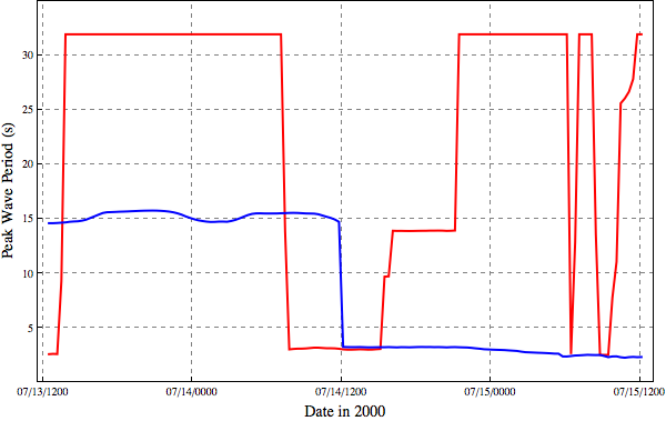
Peak wave periods (s) at a location inside Charleston Harbor for simulations with refraction (red) and without refraction (blue).
This figure shows the TPS peak periods at this point within the harbor, over the last two days of the simulation. The red line indicates results from a simulation with refraction, while the blue line indicates results from a simulation without refraction. When the refraction is enabled, the peak periods at this point are usually about 32s, meaning the peak spectral energy is located within the first, smallest frequency bin.
Note how the behavior improves when we disable the wave refraction. Then the peak periods are a relatively constant 15s, indicating that the offshore swell is propagating through the harbor to this point. When the local wind-sea takes over, then the peak periods decrease to about 3s.
These differences are confirmed by an examination of the spectra at this same geographic location:
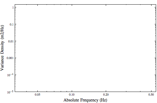
Variance density (m2/Hz) at a location inside Charleston Harbor for simulations with refraction (red) and without refraction (blue).
Note that I have plotted in log-log style to show better the results at the lowest frequencies. Again, the red line indicates the spectrum with refraction, while the blue line indicates the spectrum without refraction. The dots indicate the locations of the peak frequency.
At the higher frequencies (0.2-0.5Hz), the refraction does not change significantly the spectrum. This portion corresponds to the local wind-sea, and it evolves similarly in both simulations.
The main difference is in the lower frequencies (0.0314-0.1Hz). In the simulation without refraction, there is a clear and steady peak at about 0.065Hz, which corresponds to the swell waves with peak periods of about 15s. However, this peak is almost non-existent in the simulation with wave refraction. Instead, the wave energy is pushed down to the lowest frequency. The lowest frequency bin serves as the peak for most of the simulation, and thus we see the spikes in the peak periods to 30s or longer.
So one possible solution is to disable the wave refraction everywhere in this domain. This solution is effective in that it removes the spikes in the peak periods in the inland harbors and channels. Looking again at the peak periods corresponding to the time of the maximum significant wave heights:
Peak wave periods (s) corresponding to maximum significant wave height in a simulation without refraction.
We see clearly the dual-peak behavior in this max plot. Offshore, the peak periods correspond to the swell, and these longer waves also propagate into the harbor and between the barrier islands. Inland, the peak periods are much smaller and correspond to the wind-sea.
Of course, this is not the optimal solution. Refraction is an essential component of the nearshore wave propagation and dissipation, and so we should strive to include it in our simulations. It may be necessary to refine the mesh within these harbors and inland channels, to better represent the changes in bathymetry.
Uniform Refinement as a Possible Solution
We investigated this possible solution by creating new versions of the SC12 mesh with the resolution refined uniformly. This approach is purely academic and useful for investigation, but it has its own set of disadvantages:
First, because the resolution is refined uniformly, the resulting meshes become very large. When every triangular element is divided into four smaller elements, the overall problem size is quadrupled. Thus, the 542K-element SC12 mesh became the 2.2M-element SC12x4 mesh, which then became the 8.6M-element SC12x16 mesh. This is overkill. It is likely that the resolution needs to be increased in the nearshore regions, but not everywhere. A better implementation would increase the resolution in a way that is selective and localized to the problem areas.
Second, when the mesh is refined, the new vertices are given their properties (bathymetry, bottom friction, etc.) by interpolating linearly from the existing mesh. Thus, no new information is added to the model of the region. A better implementation would go back to the source data and re-interpolate, using a mesh-scale averaging scheme, so that the refined mesh is a more faithful representation.
So the following discussion does not represent the best solution to this problem, but rather an investigation of a possible solution. It is illustrative to look at the resolution of the refined SC12x4 mesh, in which every triangular element has been divided into four smaller elements:
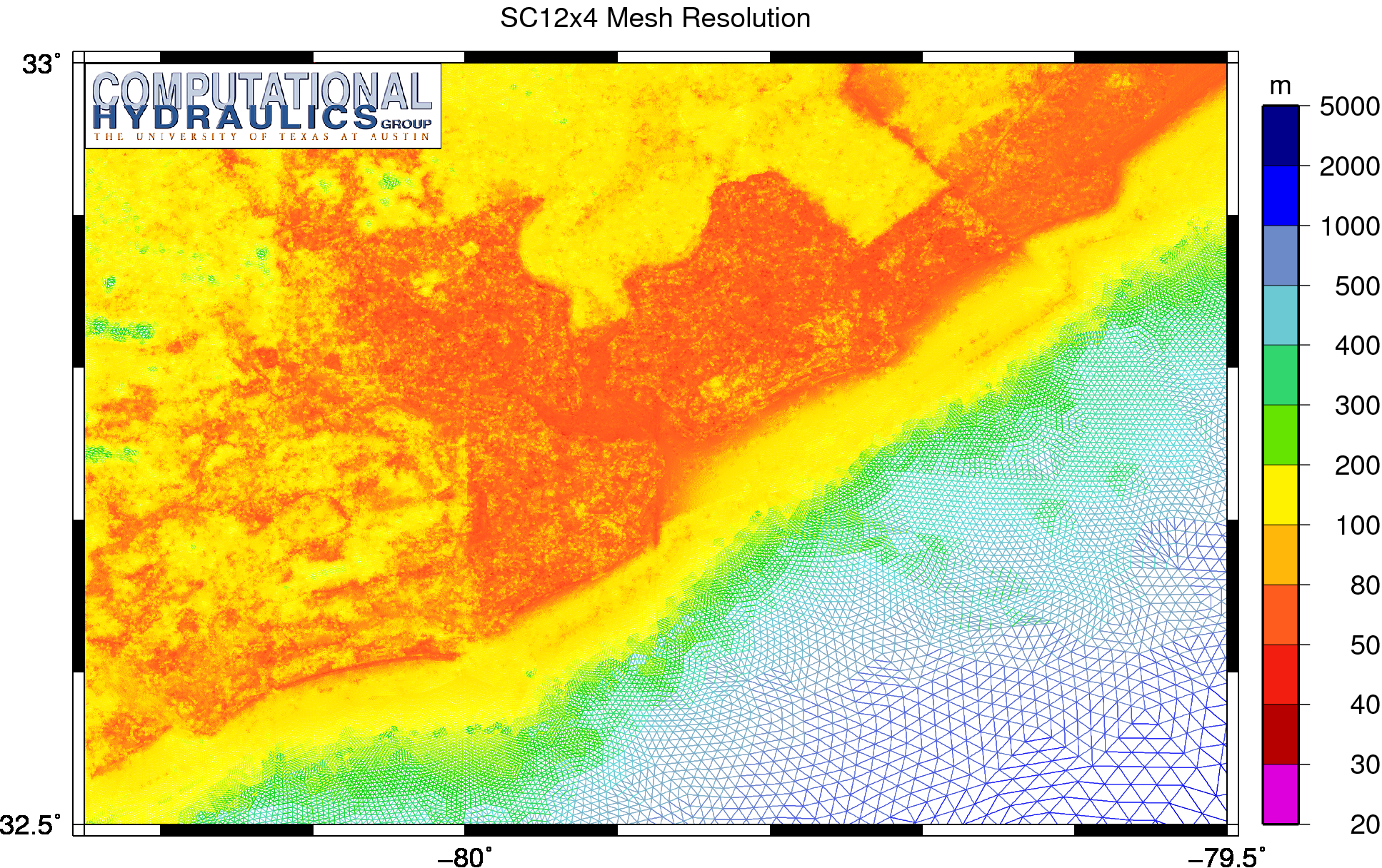
Unstructured mesh resolution (m) on the SC12x4 mesh, in which the elements have been split by four to better represent the region near Charleston, South Carolina.
Compared to a similar plot above of the original SC12 mesh, this plot of the SC12x4 mesh shows that the minimum resolution has been decreased from 100m to about 50m. This increase in resolution does improve the peak wave periods, as shown in the following image:
Peak wave periods (s) corresponding to the maximum significant wave height on the SC12x4 mesh.
The increased resolution does improve the solution, as there are fewer regions with peak periods of 30s or larger. For example, our zoom region in Charleston Harbor no longer shows the widespread spikes in the peak periods. I do not think it is a coincidence that this region also corresponds to the highest levels of resolution. The mesh sizes are smaller in Charleston Harbor than anywhere else.
But there are still regions elsewhere that do show the spikes in the peak periods. So let us try refining the mesh again. This produces the SC12x16 mesh, with resolution as shown:
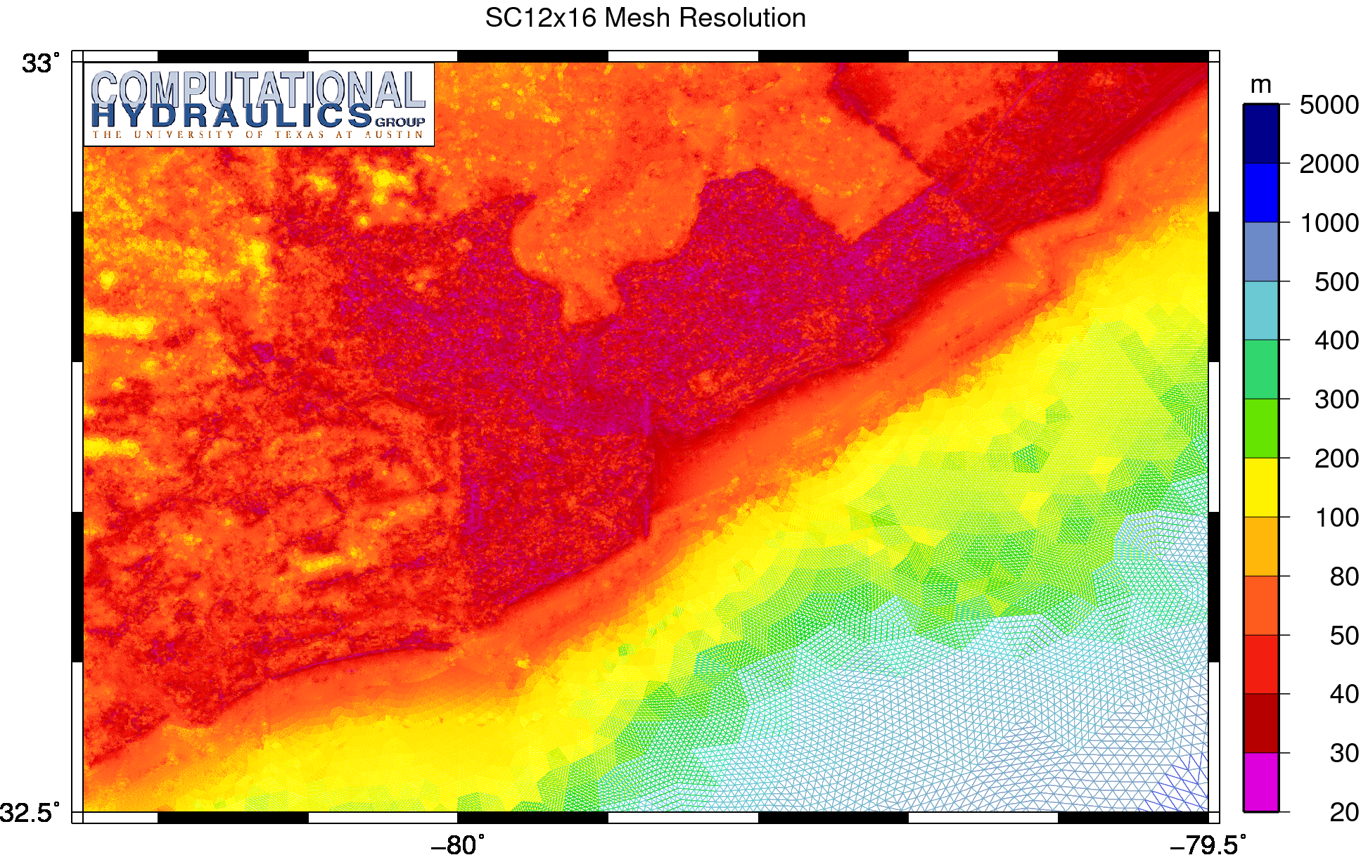
Unstructured mesh resolution (m) on the SC12x16 mesh, in which the elements have been split by 16 to better represent the region near Charleston, South Carolina.
The resolution in this refined SC12x16 mesh has been further halved, so that the minimum mesh spacing is now about 25m, and the refined mesh has 8.6M triangular elements. The resolution is so small in some regions that it causes the mesh to violate the CFL condition, and thus the time step must also be halved to maintain stability. Instead of using a 1s time step, we must use a 0.5s time step. Thus, this SC12x16 mesh is much too expensive to represent a real solution to our problem.
But it does improve the peak periods, as shown below:
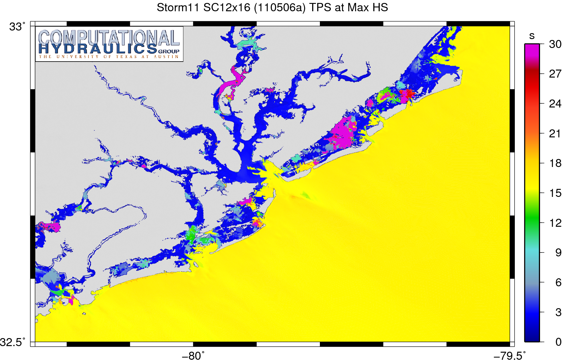
Peak wave periods (s) corresponding to the maximum significant wave height on the SC12x16 mesh.
These peak periods are now reasonable and realistic physically throughout much of the region. The increased resolution improves the behavior of the wave refraction, so that it does not push spurious energy into the lowest frequency bin. The result is a much better representation of peak periods, with far fewer purple spikes of peak periods longer than 30s.
But localized spikes still do exist. It is not worth refining further this SC12x16 mesh, because it is already unwieldy. Increased resolution does help to improve the computed solution, but it does not fix the problem.
Further Investigation of Mean Periods TMM10
We can further our investigation on this super-refined SC12x16 mesh by examining the mean wave periods (TMM10):
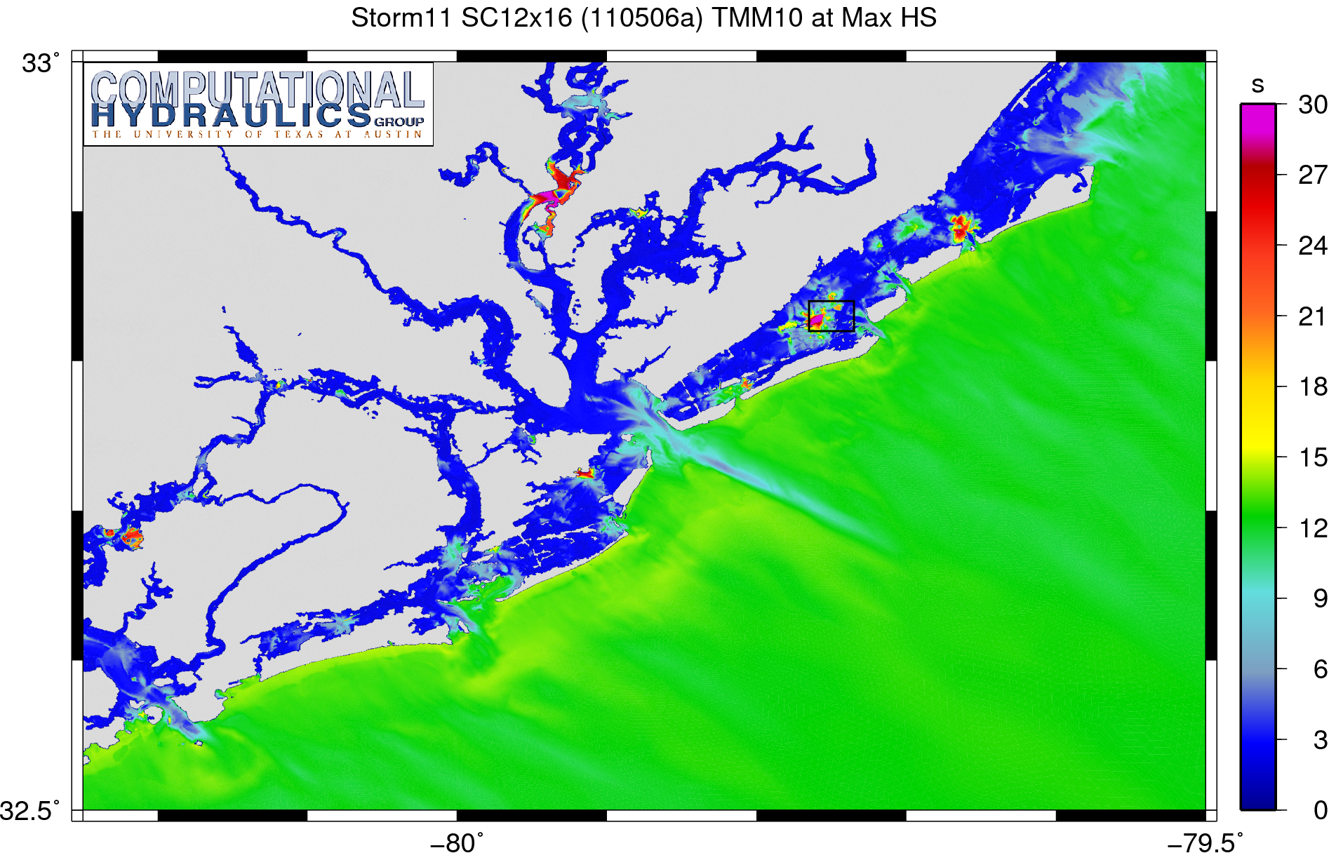
Mean wave periods (s) corresponding to the maximum significant wave height during a synthetic storm.
These mean periods correspond to the timing of the maximum significant wave heights. They are also dual-peaked, with values of about 12s offshore and values of about 3s behind the barrier islands and inland.
Note that there are spikes in these mean periods, too, but they are even more localized than in the peak periods. They should give us a good idea of where exactly in the mesh are the trouble spots located.
For example, the black square in the above image denotes the region behind the Isle of Palms, where several bays/sounds (Gray Bay, Hamlin Sound, Copahee Sound, and Bullyard Sound) are connected to the ocean via the Dewees and Capers Inlets. There are a few channels that connect everything in this region, and the coastal water way cuts through it. However, for the most part, the bathymetry is very shallow.
As shown in the animation below, the mean periods are generally fine in this region during the simulation:
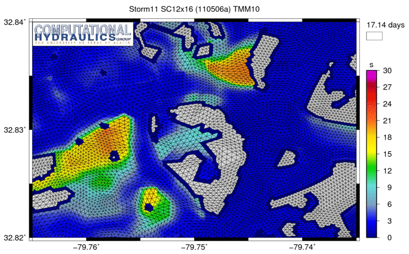
Mean wave periods (s) behind the Isle of Palms during a synthetic storm.
At normal, low-tide conditions, the channels are well-defined, and the solution is reasonable. However, as the storm moves through the region, it floods the marshes in the region. At the edges of these marshes, where the bathymetry changes rapidly from the relatively deeper channels to the relatively shallow floodplains, is where the mean periods become unrealistic physically. We see mean periods of 20s or longer.
This spurious behavior is similar to the earlier problems we observed with wave refraction on coarse meshes in deep water. The problem usually occurs at one or a few vertices where the bathymetry is changing too rapidly for the mesh to resolve properly. SWAN refracts too much energy to these vertices, resulting in spikes or peaks in the computed solution. In this case, we did not see spikes in the significant wave heights, because they were depth-limited. But we do see spikes in the wave periods.
Looking at the bathymetry and topography, even on this super-refined mesh, it is easy to see the problem areas:
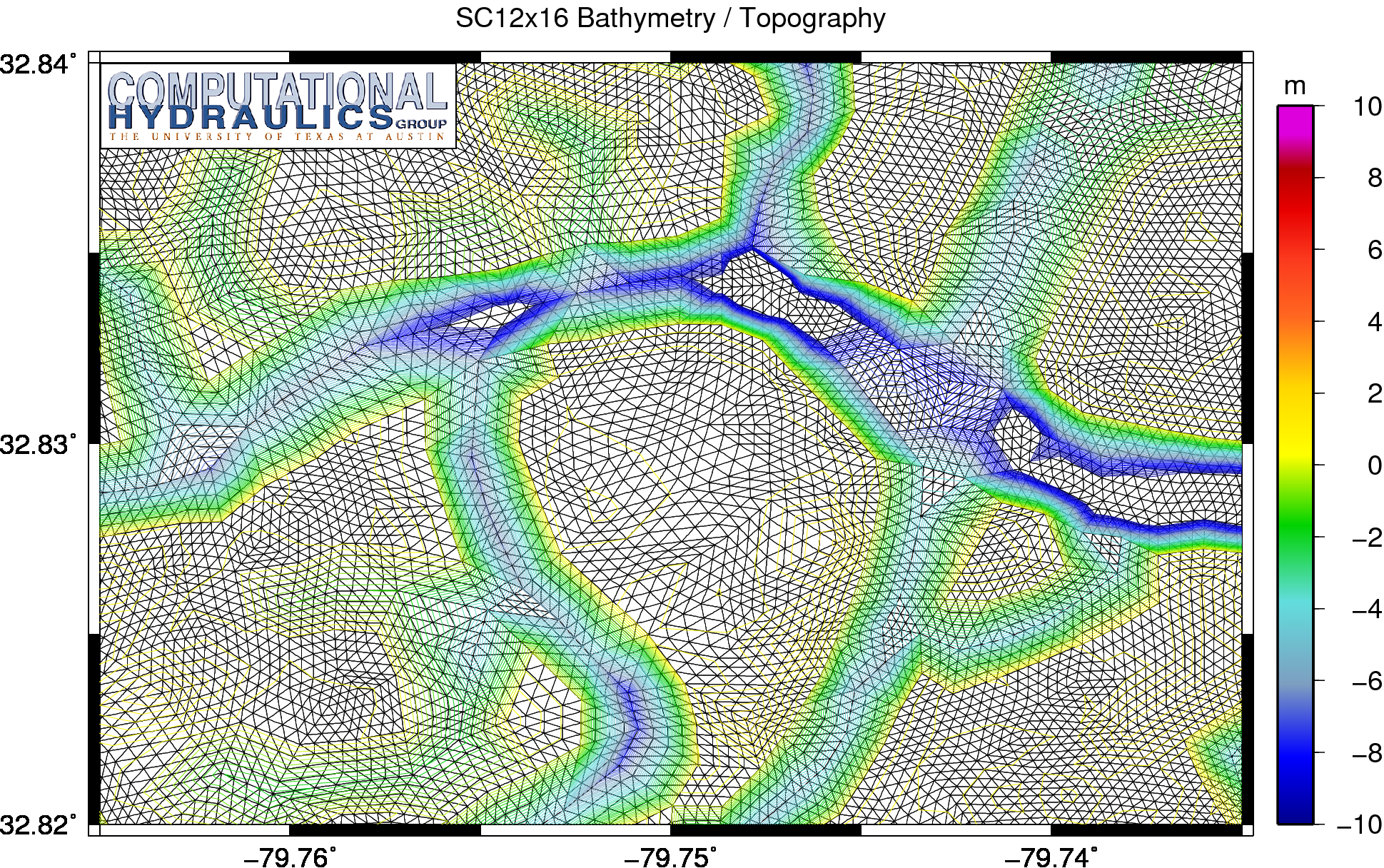
Bathymetry and topography (m) on the SC12x16 mesh behind the Isle of Palms.
The spikes in the periods correspond to the regions with the large gradients in the bathymetry, such as in the middle-left of this image (approximately 79.755W, 32.83N). The bathymetry changes by 12m over only 3-4 elements.
As noted above, although we increased the resolution on this SC12x16, so that the mesh sizes range down to about 25m, we did not add any new information because we interpolated linearly from the original mesh. In fact, the bathymetry and topography is identical on the original SC12 mesh:
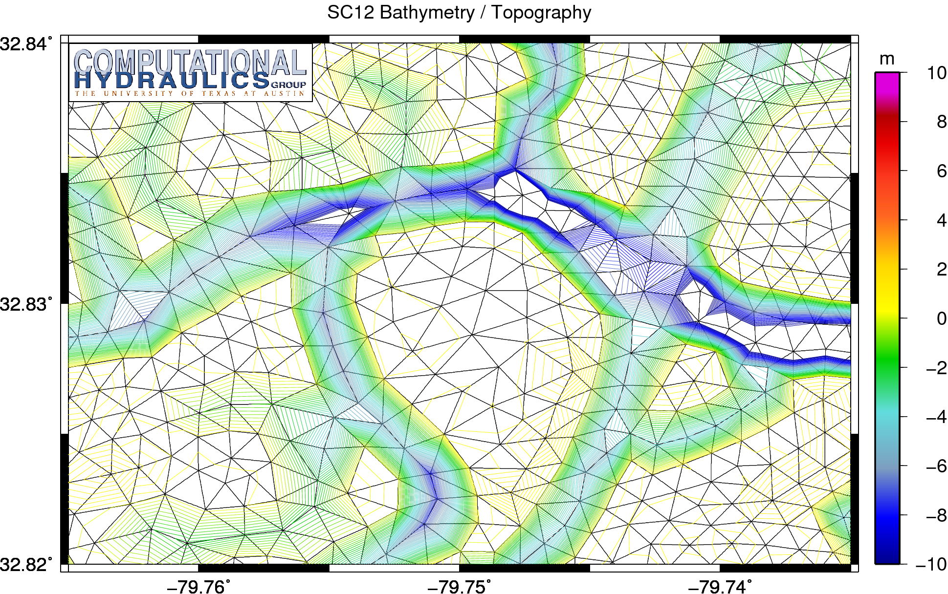
Bathymetry and topography (m) on the SC12 mesh behind the Isle of Palms.
The mesh sizes may have decreased as we refined uniformly the SC12 mesh, but the representation of the bathymetry and topography did not improve, because we interpolated linearly from the original mesh. The smaller mesh sizes did have a positive effect, because the spurious peak periods did become more localized as the mesh was refined, but refinement was not enough to remove entirely the problem areas. Even on the super-refined SC12x16 mesh, there were still a few regions with peak periods of 30s or longer.
Thus, wave refraction in SWAN requires meshes that are highly-resolved and smooth. The local mesh resolution must be adequate to capture the small-scale features and gradients in the bathymetry, and it must be applied using a mesh-scale averaging, so that the representation is smooth in the mesh. Otherwise, SWAN will refract too much wave energy to too few vertices, resulting in spikes in the computed solution.
Future work should concentrate on the development of guidelines for the generation of unstructured meshes for use with SWAN. Perhaps the problem can be reproduced on an idealized test mesh, and then investigated further. It would be great to know exactly the gradients and conditions that cause this problematic behavior, so that they can be avoided as the meshes are generated.