Kalpana converts ADCIRC output files in netCDF format to Google Earth (kmz) or GIS shapefiles for use with conventional GIS software. The latest version of the code is maintained at our GitHub repository: https://github.com/ccht-ncsu/Kalpana.
Command line arguments control the way it produces output, including the number of contour levels, their values, and the color scale. When these specifications are absent from the command line, it uses reasonable default settings so in many cases only a few of the available command line options will be used for any particular plot.
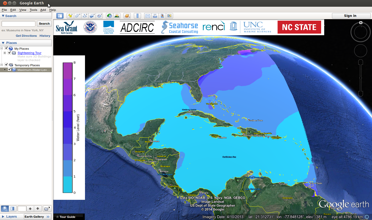
Visualization of Maximum Water Levels along the North Carolina coast during Hurricane Arthur (2014) using polygon shapefiles created by Kalpana with ArcGIS satellite imagery.
Command Line Options
The command line interface to kalpana is as follows:
python ./kalpana.py --filetype [ARGUMENTS]
The only strictly required input to Kalpana is the file type:
--filetype: different ADCIRC file types are designated by their default file names. Supported file types include bathytopo, maxele.63.nc, maxwvel.63.nc, swan_HS_max.63.nc, swan_TPS_max.63.nc, fort.63.nc, fort.74.nc, swan_HS.63.nc, swan_TPS.63.nc, and swan_TMM10.63.nc. The time-varying files (i.e., the last five in the preceding list) can be only be converted to shapefile format, but the maximum values files can be converted to either Google Earth or shapefile format. If the --filetype parameter is set to bathytopo, then the data are read from a maxele.63.nc file by default, although any other ADCIRC netCDF output file containing bathytopo data may be specified using the --filename parameter described below.
The optional arguments for Kalpana are as follows:
--viztype: The default visualization type is kmz, which is the compressed file format used by Google Earth. The output from Kalpana consists of a .kml file along with the image overlay files that accompany it. In order to get the actual kmz file, the analyst must zip up the component files, including the kml file into a zip file and give it the .kmz extension.
If shapefiles are produced, the output from Kalpana includes the following files: .cpg, .dbf, .lyr, .mxd, .prj, .shp, and .shx. The time varying output types can only be converted to shapefiles, not kmz files. The min/max file types can be converted to either shapefiles or kmz files.
--lonlatbox: When generating `kmz` output, there is a limit to the number of vertices in a single polygon, and this limit becomes relevant to high resolution mesh regions. As a result, Kalpana bins the vertices and computes polygons in the bins when preparing a visualization in kmz format. For meshes centered on North Carolina, the --code is set to “36 33.5 -60 -100” (northern latitude extent, southern latitude extent, eastern longitude extent, western longitude extent). This is also the default value. A more detailed description is provided in the Developing Kalpana page.
--subplots: The subplots argument is necessary when creating kmz output using bins as described above for the --latlonbox argument. Valid values are “yes” and “no”.
--lonlatbuffer: The buffer value is a real number used to create overlap in the bins for kmz creation as described in the previous two command line argument descriptions. This value can generally be set to 0. The default value is 0.
--palettename: Each file type has a default color palette for creating the color bar and coloring the contours. The analyst can also specify the color palette by supplying the name of the corresponding .pal file with this argument. A .pal file provides integer RGB (red green blue) values for each color in the scale with the scale being normalized from zero to one. An example of a palette file, alt-water-level.pal is as follows:
PALETTE

1

"temperature.c3g" 19

0 0.0 1.0

0.0 30 92 179

0.055 23 111 193

0.1117 11 142 216

0.1667 4 161 230

0.2217 25 181 241

0.2783 51 188 207

0.3333 102 204 206

0.3883 153 219 184

0.445 192 229 136

0.5 204 230 75

0.555 243 240 29

0.6117 254 222 39

0.6667 252 199 7

0.7217 248 157 14

0.7783 245 114 21

0.8333 241 71 28

0.8883 219 30 38

0.945 164 38 44

1.0 164 38 44
The code itself only actually uses the data from line 5 through the end of the file.
--polytype: Kalpana generates polyline as well as polygon files. The default is polygon. The polyline feature has not been fully implemented in the kmz format.
--storm: The name of the storm, event, or data set can be set with this parameter for use in labeling the resulting visualizations.
--outputfile: Each of the file types that Kalpana processes has a default output file name which can be overridden with this command line argument.
--contourlevels: If a custom set of contour levels is required, these levels can be set on the command line, enclosed in quotation marks so they are passed to the code as a single argument. Kalpana also sets reasonable default values for the contour levels of each file type.
--contourrange: As a shortcut when setting contour levels that are evenly spaced, a minimum value, maximum value, and increment value can be specified. Kalpana computes the intermediate values and generates contours at each value in the resulting range. If both a contour range and individual contour levels are specified, the contour levels take precedence.
--units: The default units system for presentation of results is the same as the units system of the output data from ADCIRC, that is, SI units. If the English system is required (e.g., presenting water surface elevation in feet instead of meters), this argument can be set to “english”. The labels for the units on the colorbars will be adjusted accordingly.
--datumlabel: The default datum label for elevation contours is “MSL”, but this argument can be used to set any arbitrary label, e.g., “NAVD”.
--logofile: A logo can be displayed at the top left corner of the Google Earth window by setting the name of the file using this argument. By default, Kalpana will try to load a file named logo.png from the current working directory where it is executed. If --logofile is set to “none” or “null“, no logo will be displayed.
--logodims: The size of the logo in the x and y directions can be set as a fraction of the display window (this is the default, with the fractions set to “0.85 0.08“) or as a certain number of pixels. Enclose the two dimensions in quotation marks so they are passed as a single argument to the code.
--logounits: The size of the logo overlay can be specified as a percent of the window size with --logounits fraction (this is the default if left unspecified), or they can be set as a certain number of pixels with --logounits pixels.
--ticks: By default, the color scale is labeled with the same values as the contour levels. However, if there are many contour levels, or the contour levels are unevenly spaced with high resolution in one particular area of the color scale, then the tick labels can overlap. The `--ticks` option allows the analyst to specify where the tick labels appear on the color scale to avoid unsightly and/or confusing overlap between tick labels.
--filename: The default file name is the same as the file type. In certain cases it may be preferable to specify the file name as well; for example, the ADCIRC output file may have the full path prepended to it.
Examples
The following examples were taken from the real time output data for Arthur 2014 advisory 12. These output data can be downloaded from the public THREDDS Data Server at the Renaissance Computing Institute (RENCI).
1. Water Surface Elevation
a. Maximum Water Levels (in feet above MSL) visualized in Google Earth with logo.
This example describes the visualization of the maximum water levels along the NC coast during Hurricane Arthur Advisory 12. The following command will create a Google Earth visualization of the maxele.63.nc file with units set to feet, the datum left at the default value of “MSL“, the contour levels set to every half foot from 0 to 5 feet, an analyst-specified contour color palette named alt-water-level.pal, the default file name being set to maxele.63.nc to match the specified file type, and a logo image across the top of the visualization loaded from a file called logo.png:
python ./kalpana.py --storm arthur --filetype maxele.63.nc --polytype polygon --viztype kmz --subplots yes --lonlatbox '36 33.5 -60 -100' --lonlatbuffer 0.0 --contourrange "0 5 0.5" --units english --palettename alt-water-level.pal
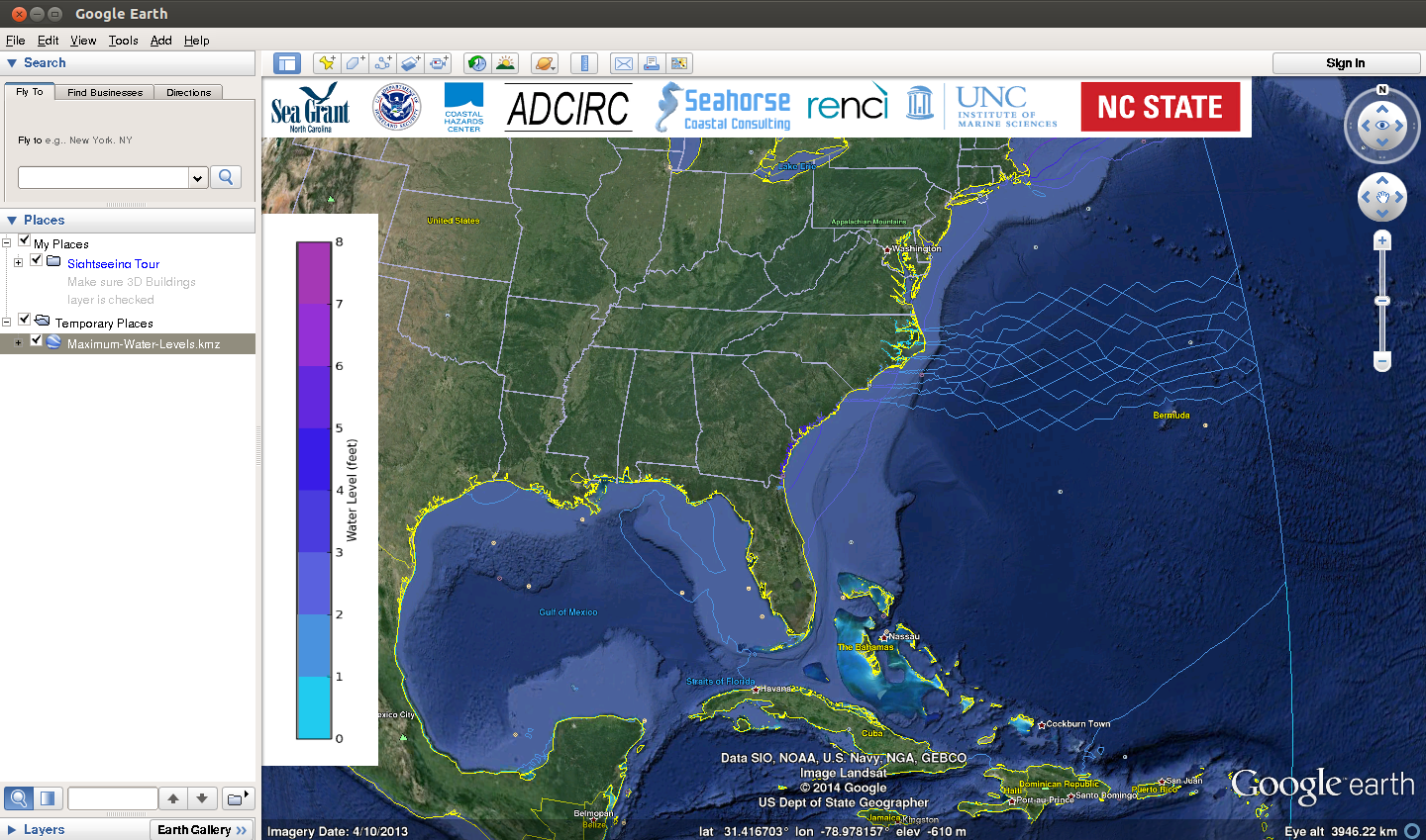
The output from the above command for Example 1a was written to the default file name Maximum-Water-Levels.kml and is shown below. If the --filetype parameter is not specified, then the maxele.63.nc is loaded by default.
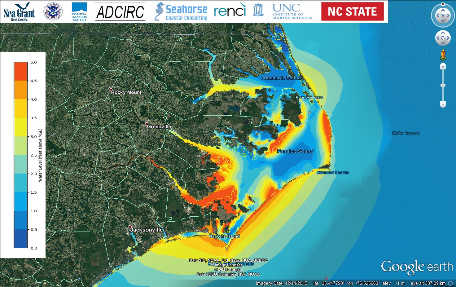
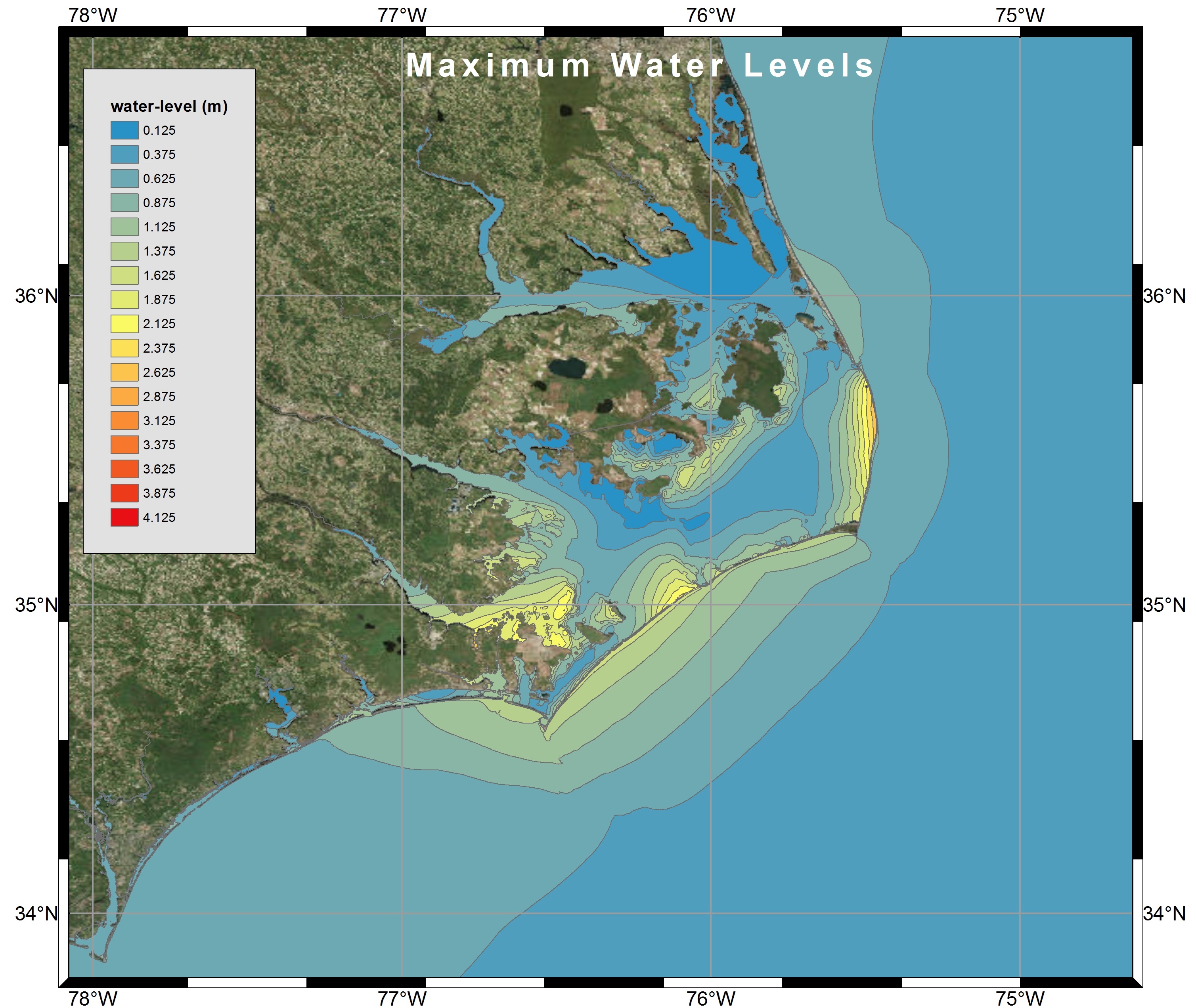
Example 1a: Maximum water levels (feet) along the NC coast during Hurricane Arthur Advisory 12, visualized in Google Earth.
b. Maximum Water Levels (in m above MSL) visualized in Google Earth without logo.
Example 1a can be modified by turning the logo bar completely off, labelling the datum “mean sea level“, displaying the results in the default SI units system, adjusting the contouring range accordingly, and writing the results to a custom output file name to avoid overwriting the previous results:
python ./kalpana.py --storm arthur --filetype maxele.63.nc --polytype polygon --viztype kmz --subplots yes --lonlatbox '36 33.5 -60 -100' --lonlatbuffer 0.0 --contourrange "0 2 0.25" --palettename alt-water-level.pal --logofile none --outputfile withoutlogo --datumlabel "mean sea level"
The command above for Example 1b produced a file called withoutlogo.kml and is shown below.
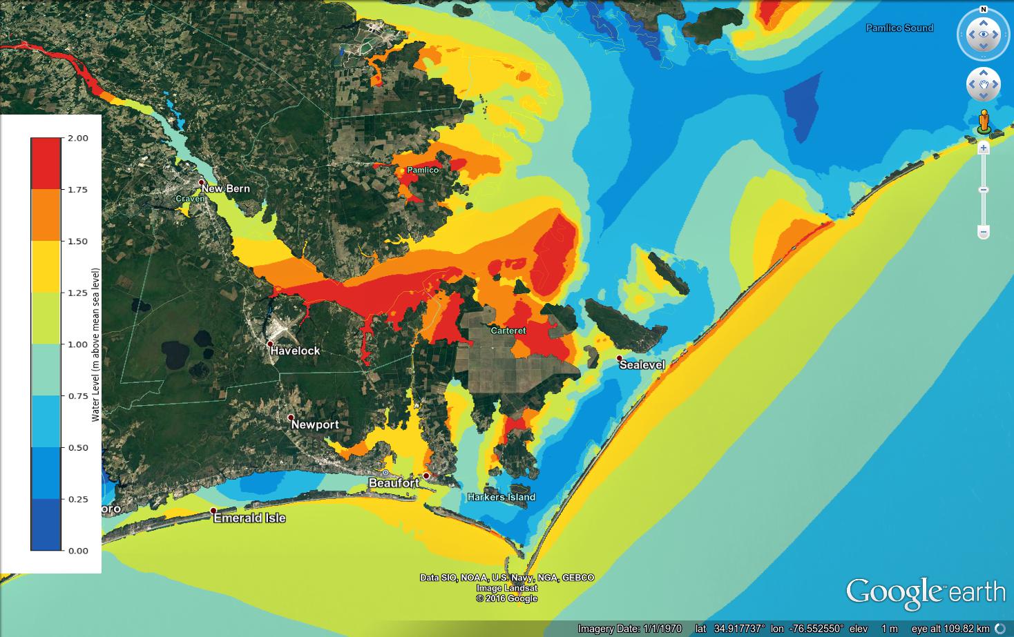
Example 1b: Same as Example 1a above, but with changes to the logo, units, and contour range.
c. Maximum Water Levels (in feet) visualized in ArcGIS via a polygon shapefile.
A further Example 1c for the `maxele.63.nc` file is provided below for producing a shapefile similar to Example 1b, but with fewer parameters because shapefiles are not subject to the limitation on the maximum number of vertices in a polygon the way kmz files are:
python ./kalpana.py --storm arthur --filetype maxele.63.nc --polytype polygon --viztype shapefile --contourrange "0 5 0.5" --units english
Example 1c produced a shapefile (an accompanying files) using the default file name:
water-level.cpg

water-level.prj

water-level.shx

water-level.dbf

water-level.shp
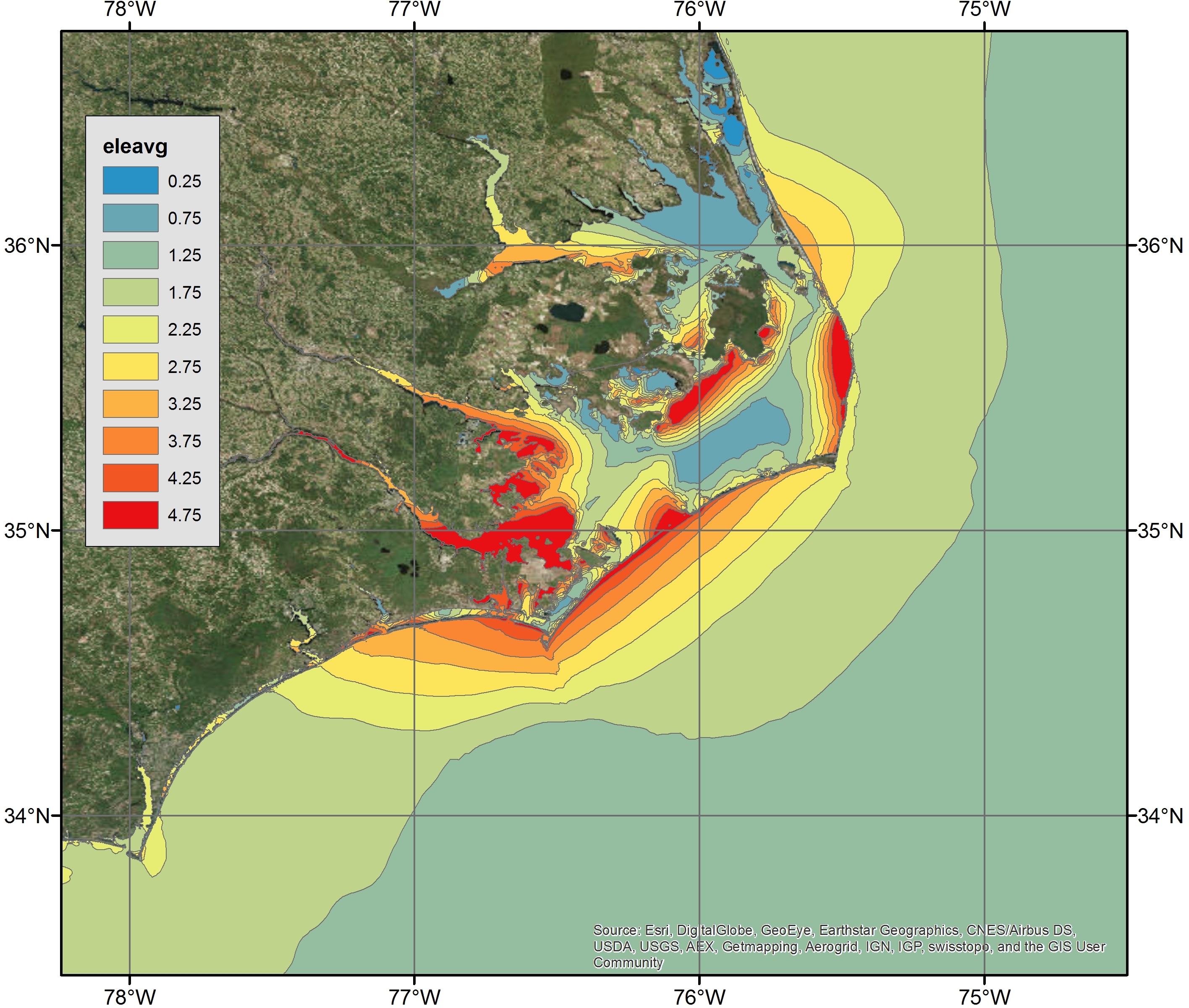
Example 1c: Maximum Water Levels (feet) along the NC coast during Hurricane Arthur Advisory 12 visualized via polygon shapefiles with ArcGIS satellite imagery
d. Time series of water surface elevation (in feet) visualized via a time varying shapefile.
The final water surface elevation example operates on the full domain time series of water surface elevation (i.e., the fort.63.nc file) to produce a time varying shapefile:
python ./kalpana.py --storm arthur --filetype fort.63.nc --polytype polygon --viztype shapefile --subplots no --contourrange "0 5 0.5" --units english
The image below shows the water levels along the NC coast during Hurricane Arthur Advisory 12 at an intermediate time step (07/04/2014 0900 UTC) during the simulation period.
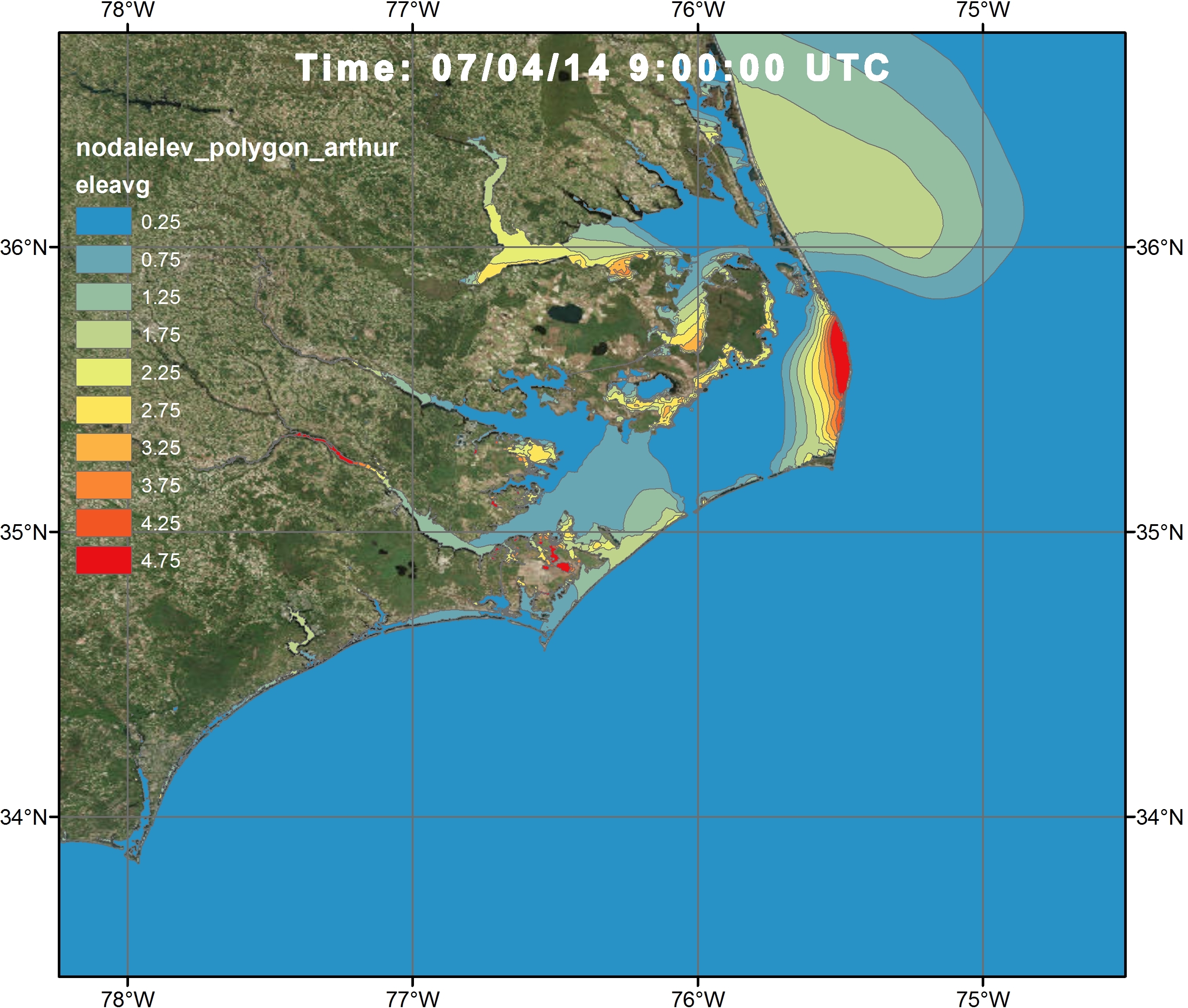
Example 1d Visualization of the water levels (feet) along the NC coast during Hurricane Arthur Advisory 12 at 07/04/14 0900 UTC via a time varying shapefile with ArcGIS satellite Imagery
2. Wind Speed
a. Maximum Wind Speeds (in mph) visualized in Google Earth with logo.
This example provides a visualization of the ADCIRC maximum wind speed file (i.e., the maxwvel.63.nc file) in Google Earth with the command line options given below:
python ./kalpana.py --storm arthur --filetype maxwvel.63.nc --polytype polygon --viztype kmz --subplots yes --lonlatbox '36 33.5 -60 -100' --lonlatbuffer 0.0 --contourrange "0 60 5" --units english --palettename alt-water-level.pal
Care should be taken when converting wind velocity or maximum wind speed files to vector formats because of the wind reduction factors over land. The resulting patchy wind speed contours result in intricately complex polygons that may take much longer to generate than for other output file types. Example 2a above took over two hours to compute (compared with less than 5 minutes for the other examples).
Example 2a: Maximum wind speeds (mph) along the NC coast during Hurricane Arthur (2014) Advisory 12, as visualized in Google Earth.
b. Maximum Wind Speeds (in mph) visualized in ArcGIS via a polygon shapefile
This example provides a visualization of the ADCIRC maximum wind speed file (i.e., the maxwvel.63.nc file) in ArcGIS with the command line options given below:
python ./kalpana.py --storm arthur --filetype maxwvel.63.nc --polytype polygon --viztype shapefile --contourrange "0 90 5" --units english
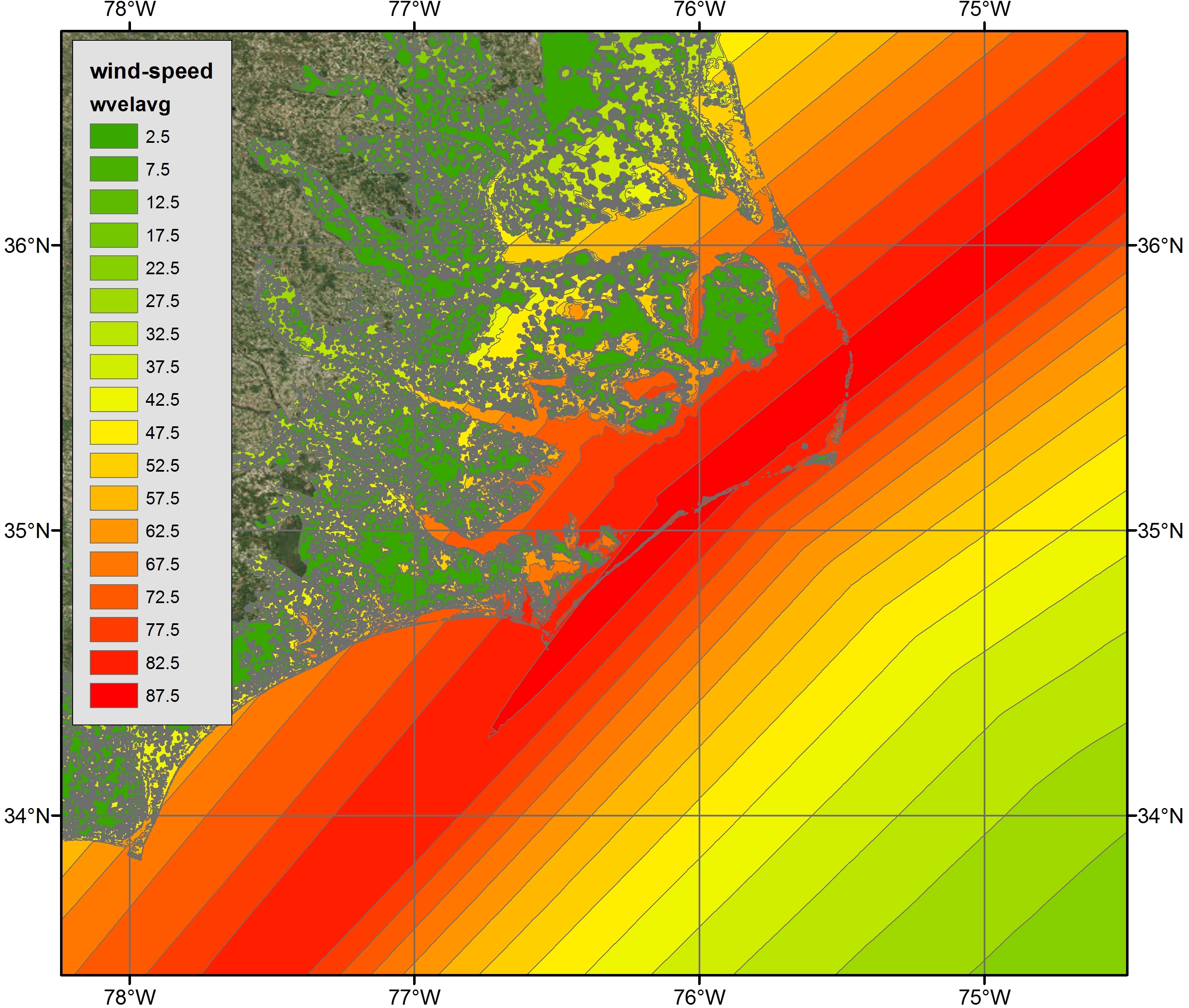
Example 2b: Maximum Wind Speeds (mph) along the NC coast during Hurricane Arthur Advisory 12 visualized via polygon shapefiles with ArcGIS satellite imagery
3. Wave Height
a. Maximum Significant Wave Heights (in m) visualized in Google Earth.
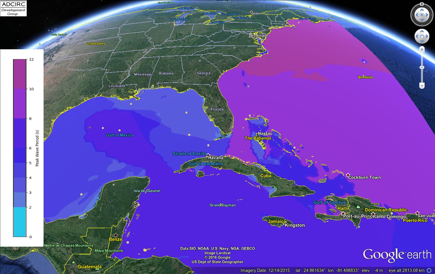
The wave height from SWAN is available as peak wave height in the swan_HS_max.63.nc file, or in the time varying full domain wave height file, swan_HS.63.nc. Example 3a below is a Google Earth visualization of the SWAN maximum wave height file using filled polygons, default SI units with the contour levels explicitly specified and evenly set from 0 to 12m, an analyst specified color scale in the file alt-water-level.pal, an analyst specified logo in the file adg_logo.jpg with logo dimensions set to 10% of the vertical and 10% of the horizontal space in the visualization:
python ./kalpana.py --storm arthur --filetype swan_HS_max.63.nc --polytype polygon --viztype kmz --subplots yes --lonlatbox '36 33.5 -60 -100' --lonlatbuffer 0.0 --contourlevels "0 1 2 3 4 5 6 7 8 9 10 11 12" --palettename alt-water-level.pal --logofile adg_logo.jpg --logodims "0.1 0.1"
Example 3a above produced a kml file with the default file name Maximum-Wave-Height.kml and is shown below.
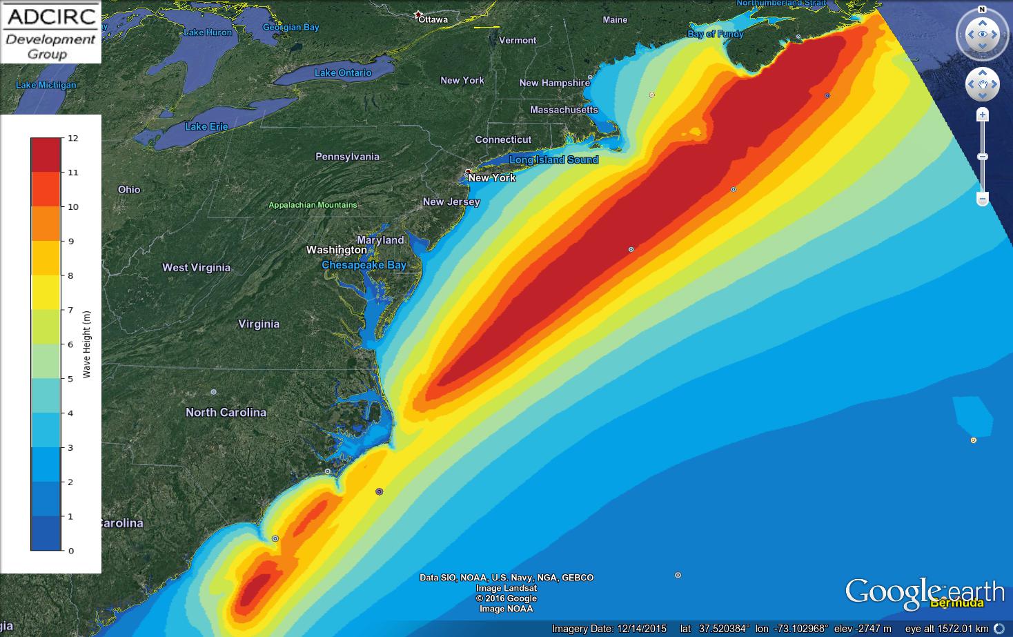
Example 6: Maximum Significant Wave heights (m) during Hurricane Arthur (2014) Advisory 12, as visualized in Google Earth.
b. Maximum Significant Wave Heights (in m) visualized in ArcGIS via a polygon shapefile.
Example 3b shows the same data being written to a polygon shapefile:
python ./kalpana.py --storm arthur --filetype swan_HS_max.63.nc --polytype polygon --viztype shapefile --subplots no --contourlevels "0 1 2 3 4 5 6 7 8 9 10 11 12"
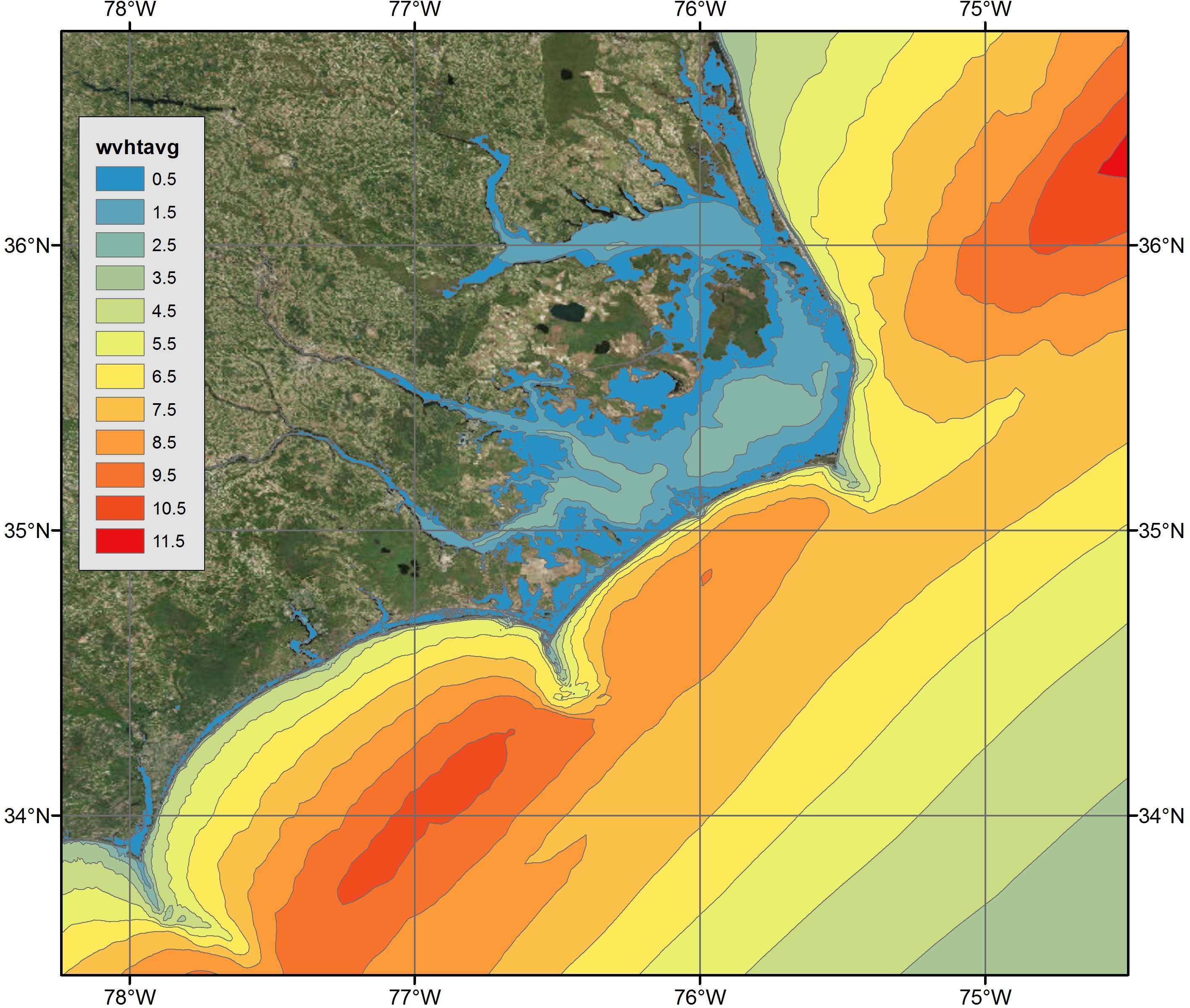
Example 3b: Maximum Significant Wave Heights (m) along the NC coast during Hurricane Arthur Advisory 12 visualized via polygon shapefiles with ArcGIS satellite imagery
c. Time series of significant wave heights (in m) visualized in ArcGIS via a time varying polyline shapefile.
Finally, Example 3c shows the time varying full-domain ADCIRC+SWAN wave height with polylines, as opposed to polygons, in shapefile format:
python ./kalpana.py --storm arthur --filetype swan_HS.63.nc --polytype polyline --viztype shapefile --subplots no --contourlevels "0 1 2 3 4 5 6 7 8 9 10 11 12"
The image below shows the significant wave heights along the NC coat during Hurricane Arthur Advisory 12 at an intermediate time step (07/04/2014 0900 UTC) during the simulation period.
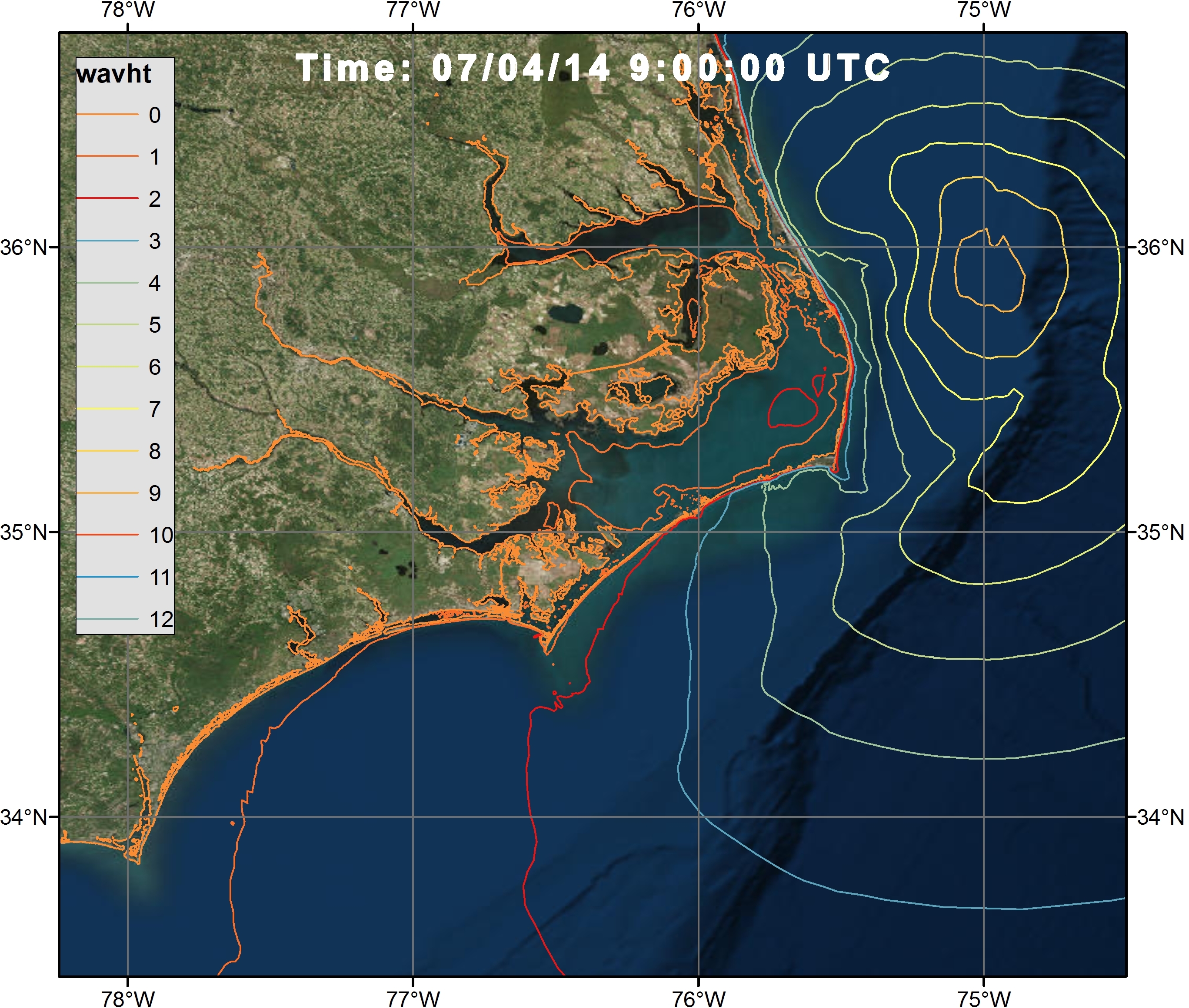
Example 3c: Visualization of the significant wave heights (m) during Hurricane Arthur Advisory 12 along the NC coast at 07/04/14 0900 UTC via a time varying polyline shapefile with ArcGIS satellite Imagery
4. Wave Period
a. Maximum Peak Periods (in s) visualized in Google Earth.
The ADCIRC+SWAN full domain maximum wave period file swan_TPS_max.63.nc is visualized below in Example 4a, where the input file name is set to a non-default value, the contour levels are specified explicitly and are not uniformly spaced, the default color scale is used, and an analyst specified logo is provided in a file named adg_logo.jpg with dimensions of “90 55” in units of pixels:
python ./kalpana.py --storm arthur --filename arthur12-swan_TPS_max.63.nc --filetype swan_TPS_max.63.nc --subplots yes --contourlevels "0 2 3 4 5 6 8 10 12" --logofile adg_logo.jpg --logodims "90 55" --logounits pixel
The results are shown below:
Example 9: Maximum peak wave periods (s) during Hurricane Arthur (2014) advisory 12, as visualized in Google Earth.
b. Maximum Peak Periods (in s) visualized in ArcGIS via a polygon shapefile.
A corresponding shapefile may be produced as follows in Example 4b below:
python ./kalpana.py --storm arthur --filetype swan_TPS_max.63.nc --polytype polygon --viztype shapefile --subplots no --contourlevels "0 2 4 6 8 10 12 14 16 18"
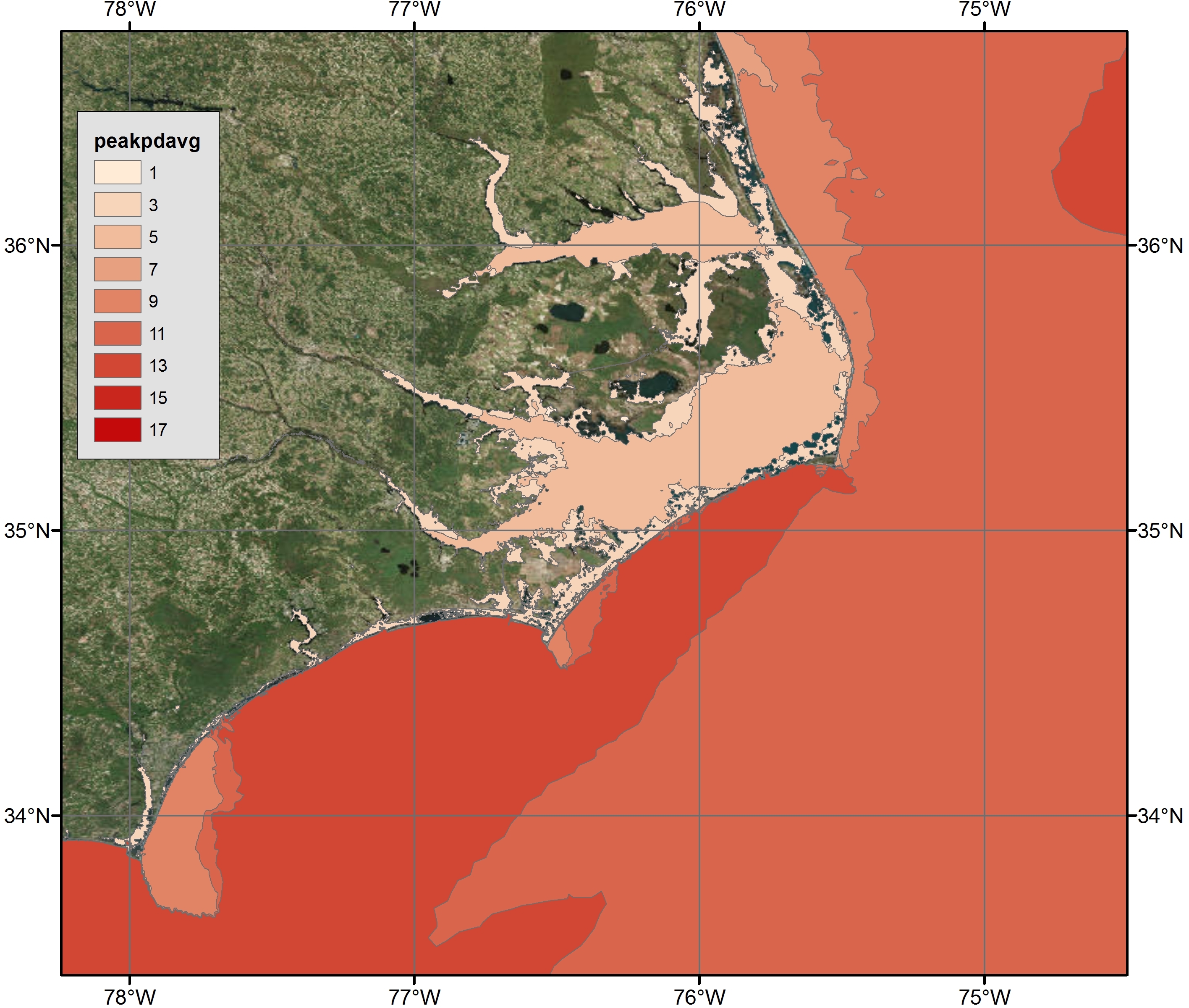
Example 4b: Maximum Peak Wave Periods (s) along the NC coast during Hurricane Arthur Advisory 12 visualized via polygon shapefiles with ArcGIS satellite imagery
5. Bathymetry/Topography
a. Bathymetry/Topography visualized in Google Earth.
The final Examples 5a and 5b depict the visualization of the ADCIRC mesh bathymetry and topography in Google Earth and ArcGIS respectively. This example loads the bathy/topo elevations from a maxele.63.nc file, uses an analyst-specified color palette called mesh-bathy_bluegreen.pal along with a carefully matched set of unevenly spaced contour levels from -20m to 100m, an analyst specified set of unevenly spaced tick labels (to avoid bunching up the tick labels near mean sea level, the default logo, the default datum label, and the defailt SI units:
python ./kalpana.py --storm arthur --filetype bathytopo --polytype polygon --viztype kmz --subplots yes --lonlatbox '36 33.5 -60 -100' --lonlatbuffer 0.0 --contourlevels "-20 -10 -5 -2 -1 -0.5 -0.2 -0.1 0.0 0.0001 0.1 0.2 0.5 1 2 5 10 20 50 100" --filename maxele.63.nc --palettename mesh-bathy_bluegreen.pal --ticks "-20 -10 -5 0 2 5 10 20 50 100"
The results of Example 5a are shown below.
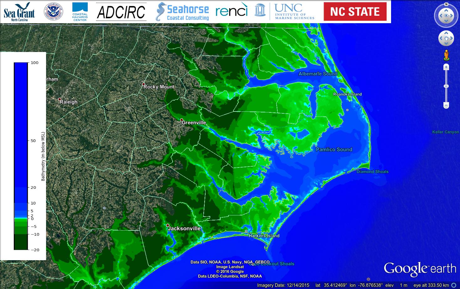
Example 5a: Bathymetry and topography (m) for the high-resolution mesh describing the North Carolina coast visualized in Google earth.
b. Bathymetry/Topography visualized in ArcGIS via a polygon shapefile.
An equivalent shape file can be produced as shown in Example 5b.
python ./kalpana.py --storm arthur --filetype bathytopo --polytype polygon --viztype shapefile --contourlevels "-20 -10 -5 -2 -1 -0.5 -0.2 -0.1 0.0 0.0001 0.1 0.2 0.5 1 2 5 10 20 50 100" --filename maxele.63.nc
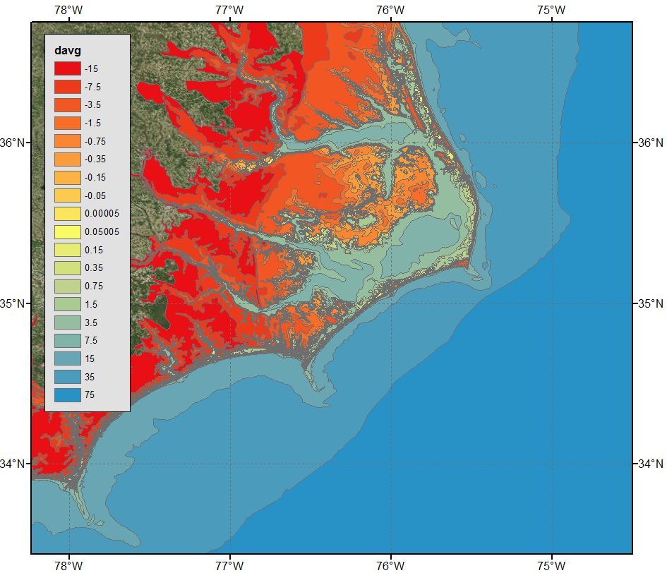
Example 5b: Bathymetry and topography (m) for the high-resolution mesh describing the North Carolina coast visualized using polygon shapefiles with ArcGIS satellite imagery.
Appendix: Troubleshooting Google Earth Errors
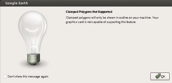
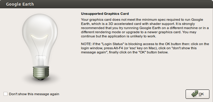
When first attempting to load the Google Earth (kmz) sample file Maximum-Water-Levels.kmz, I ran into a few perplexing issues. When Google Earth started up, it produced the error message shown below.
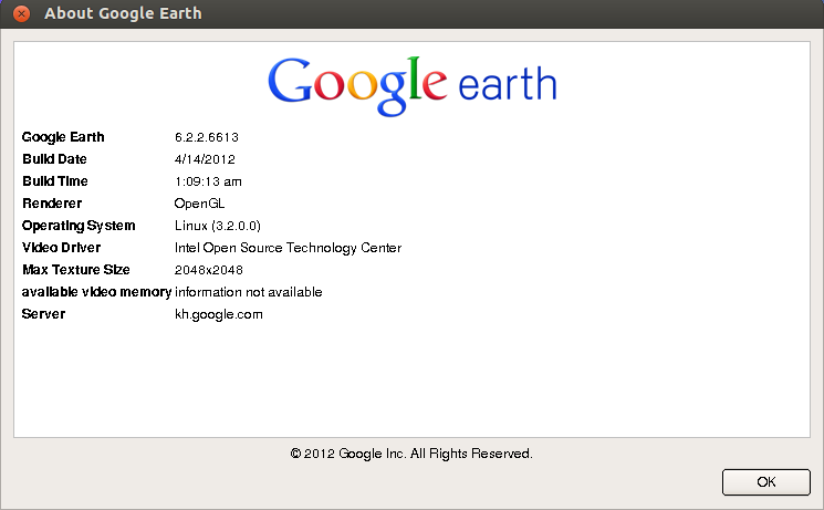
The Google Earth version information is shown below.
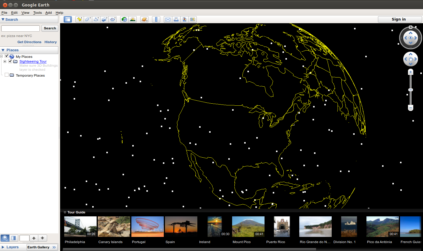
As a result of this error, when the data files were actually displayed, the contours were only shown in outline.
I upgraded to the latest available version of Google Earth (v7.1.2.2041) in the hope that this would resolve the issue.
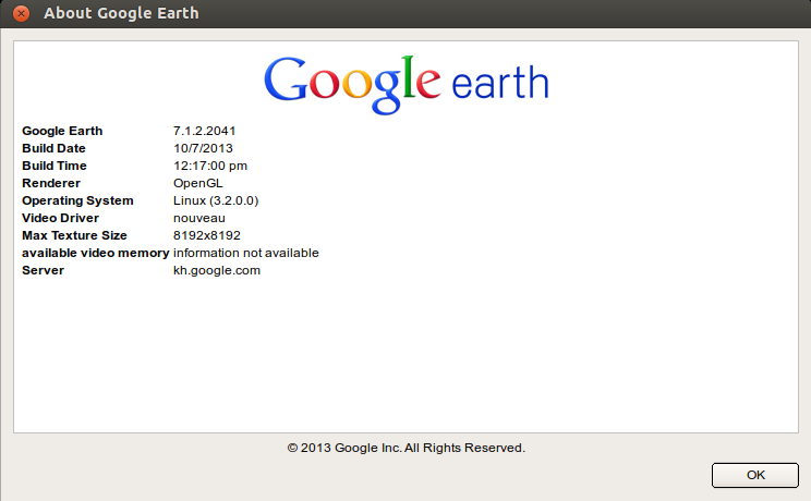
However, upgrading to the latest available version of Google Earth did not resolve the issue. Although I did get a more verbose error message with more explicit advice.
After clicking through the error message, the graphics were even less usable than in the prior version of Google Earth.
Finally, after installing a new video card in my desktop machine, the Google Earth visualization of the original kmz files (provided with the code) worked successfully.