
This document describes the methodology followed in kalpana.py for the creation of shape file and kml files. The sequence of steps involved has been grouped under related sub-headings for better comprehension. The terms in fixed width font refer to variable names in the code.
Input Data
-
ADCIRC output file in netCDF format or the corresponding OPeNDAP URL.
-
Appropriate color palette files (files with .pal extension) to specify the desired color scheme during KML creation. The palette files included with the current package are
water-level.palandwavht.pal. -
To have some control over the symbology in which the shape files are visualized in ArcGIS, .mxd and .lyr files have been created outside the code. To package them with the shape file distribution, a directory with the same name as the shape file has also been included. This directory contains a sample shape file, a .mxd and a .lyr file. Every time a new shape file with the same name is created, the previous one is overwritten. The .mxd and .lyr files is tuned to reference the current shape file (with the same base file name as the .mxd/.lyr files) within the directory. Including the .mxd and .lyr files is completely optional.
Modules
The following Python modules are used within Kalpana:
matplotlib– main python module used for data visualization.pylab– Imports plotting and numerics libraries in a single name space.shapely– used to construct geometric objects like Points, Polygons and LineStrings.fiona– for writing .shp files.netCDF4– reading and writing netCDF files.datetime– dates and time calculation, manipulation, and formatting.time– contains time related functions for measuring the performance of the code itself.numpy– to facilitate scientific computing; used primarily in Kalpana for working with n-dimensionalnumpyarrays, which are ideal for storing large amounts of data.collections– accessing OrderedDict, which is a dictionary subclass that remembers the order in which entries were added, whereas an ordinary dictionary does not do so).simplekml– writing kml (Google Earth) files.
Google Earth Vertex Limit
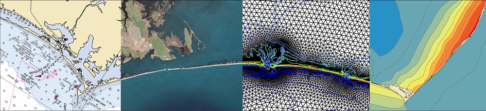
While creating the kmz files for the entire domain of the NC9 mesh for North Carolina, it was noticed that the largest polygon (corresponding to the lowest contour level) was rendered incorrectly. This was due to the number of vertices in its outer boundary being too high. It exceeded 31,000 vertices, which is the upper limit specified in Google Earth documentation for a polygon boundary to be rendered correctly.
As a solution to this issue, the entire mesh domain is divided into a series of lon-lat bins such that there are more bins in regions of higher mesh resolution. The idea is to plot contour levels and generate polygons for each of these sub domains separately and later combine them.
In the present code, the entire domain is specified using:
gdomain=[50, 5,-60,-100]
which specifies a range of latitudes from 5 degrees to 50 degrees North, and a range of longitudes from 60 degrees to 100 degrees West. The user is then prompted to enter a local box (e.g., an area of interest with a higher mesh resolution) where bins can be defined at smaller intervals. For the NC9 mesh, we have used a local box of:
gdomain=[36, 33.5,-60,-100]
This constituted the regions near and along the NC coast with high levels of resolution in this mesh. Within this local box, different lon-lat bins are created with widths of 0.5 degrees.
It is to be noted the same procedure is applicable for the visualization of results of other complex meshes. However the local box has to be chosen appropriately. Also the bins are chosen assuming that the mesh is more finely resolved in the north-south direction within the local box. This approach may cause problems while applying to a coastline which has very fine features extending along the east-west direction as well. For such applications, the local box should be selected appropriately.
General Settings for Shapefiles and KML files
Shapefiles
-
Define Spatial Reference (
crs) which specifies the ellipsoid, datum and projection used. -
Define OGR Driver (
driver).
KML files
-
Create a simplekml object (
kml). -
Define a region (
reg) with a specified lat-long box (box) and Level of Detail (LOD) (lod) (specifying the minimum and maximum pixels the kml object should occupy before it disappears). -
Creation of colorbar based on the colors specified in
hex. -
Screen Overlays are created to insert the logo and color bar into the kmz file.
Processing Input Data at Every Time Step
The following processes are repeated at every time step:
Triangulation and Contouring
If you are plotting directly for the full domain, then the triangulation (tri) and contouring (contour) is done for the full domain. Otherwise, a local mesh is created for each specified lon-lat box. The procedure for deriving a local mesh from a global mesh is explained in Appendix A. Triangulation and contouring is done separately for each local mesh using the vertex (localx, localy), element (localelements) and variable (localvar) information derived for each local mesh.
Extracting Information
The enumerate (contour.collections) gives a list of contour levels (colli) in the form of indices and contours that store all the vertices lying in that contour in the form of path objects (coll). Each contour level may have more than one path. All the paths corresponding to a single contour level can be accessed using get_paths().
For creating polylines, the vertices stored in each of the paths can be extracted using .vertices and wrapped into a shapely LineString object. For creating polygons, each of the paths can be converted into polygons (polys – a list of numpy arrays containing vertices defined for each polygon) using to`_`polygons().
Writing Shapefiles
The above set of polygons corresponding to each path is wrapped into a shapely Polygon object. An empty ordered dictionary (geoms) is defined outside the time step loop and each time step is added as a key to this dictionary. A tuple consisting of the shapely Polygon object and the corresponding minimum and maximum contour levels is stored in geoms against the appropriate time step. This step is repeated for all the contour levels. Thus geoms has the following form:
{“timestep1”:[(Polygon1,min1,max1),(Polygon2,min2.max2),(….)…] “timestep2”:[ ( ….), (…)…..]……}
Writing kml Files
-
Define a new folder (
fol) for every time step. For each contour level a multigeometry kml object (multipol) is defined as a child offoland a Python list of these multigeometry elements is created (store). A list of Python tuples (polys1) is created frompolyswhere each tuple represents a polygon. The next step is to identify the outer and inner polygons inpolys1by calculating the signed area of each polygon. Area is positive for an outer polygon and negative for an inner polygon. Outer and inner polygons are stored inouterandinnerrespectively. -
The list of outer polygons is traversed and the inner polygons which fall within each outer polygon are identified. This is done by checking if any one of the vertices on the boundary of an inner polygon falls within the outer polygon (Note: no two polygons can intersect each other since they represent contour levels). A list of the indices of inner polygons which fall within an outer polygon is stored in a Python dictionary (
topo) with the corresponding outer polygon number as keys. -
For each contour level, each of the outer polygons with all its inner polygons are stored as a child element of the corresponding multi geometry object ((
store[m]) where (m) refers to each contour level). Visibility, fill, color, outline, description etc. is defined for each multigeometry object (store[m]).
Defining Schema and Writing Shapefiles
-
The geometry (Line String, Polygon etc.) and attribute properties (name of attribute and data type (int, float etc.) corresponding to each output shapefile is defined by the schema (
schema). -
A new shapefile is opened using Fiona. The data stored in
geomcorresponding to each time step is written into this shapefile.
Creating the KMZ File
The simplekml object is saved as a .kml file. The kml file is zipped with the corresponding color bar file (ex: Colorbar-water-levels.png) and the logo (logo.png). Zipping the files is not included in kalpana.py. It can be done using the zipfile module of python.
Appendix A
Creating local mesh from the global mesh for a specified lon/lat box:
-
Define a subdomain using the bounding latitude (North and South) and longitude (East and West) values. These are defined as
LatN,LatS,LongE, andLongWrespectively. -
Specify a buffer distance to have a smooth overlap of the plots from adjacent subdomains.
-
Traverse through all the elements in the mesh. If any of the vertices of each element falls within a specified lat-long box then that element and all its vertices are considered to be within that lat-long box. The values at the corresponding indices (representing the element number or node number) in
includeele1andincludevertex1are updated to 1. -
Traverse through all elements in the mesh. Check the value of
includevertex1for all the vertices for each element. If the value is 1 for any of them updateincludeele2andincludevertex2at the corresponding vertices to 1 like in Step 3. -
Traverse through all the nodes in the mesh. Check the value of
includevertex2for each node. If the value is 1 then consider that node to be in the new local mesh and include its latitude and longitude values inlocallatandlocallonrespectively. Renumber the vertices that fall in the local mesh and create a look up table with the global and local node numbers of each vertex. Also store the value of the ADCIRC output variable corresponding to these vertices invarlocal. -
Repeat step 5 for all the elements of the domain. For each element check if
includeele2at the corresponding element number. If it is 1 then append a tuple containing the coordinates of each of its vertices to the listlocalelem. -
Return
locallat,locallon,localelem,varlocal.