Downscaling with Head Loss due to Land Cover in Kalpana | Coastal & Computational Hydraulics Team

Originally developed as a tool for visualizing ADCIRC output, Kalpana has evolved to include methods for downscaling ADCIRC water elevation results. The first method, now referred to as the static method, extrapolated ADCIRC water elevations horizontally until intersecting an equivalent DEM elevation. More information about the static method and about downscaling ADCIRC results with Kalpana can be found on an earlier post.

The static method has proven to be a useful tool but incorporates minimal physics. Therefore, a new method, referred to as the head loss method, has been introduced to include energy dissipation due to land cover during overland flow events. In this page, we describe the theory of the head loss method and provide examples for how to apply it using Kalpana.

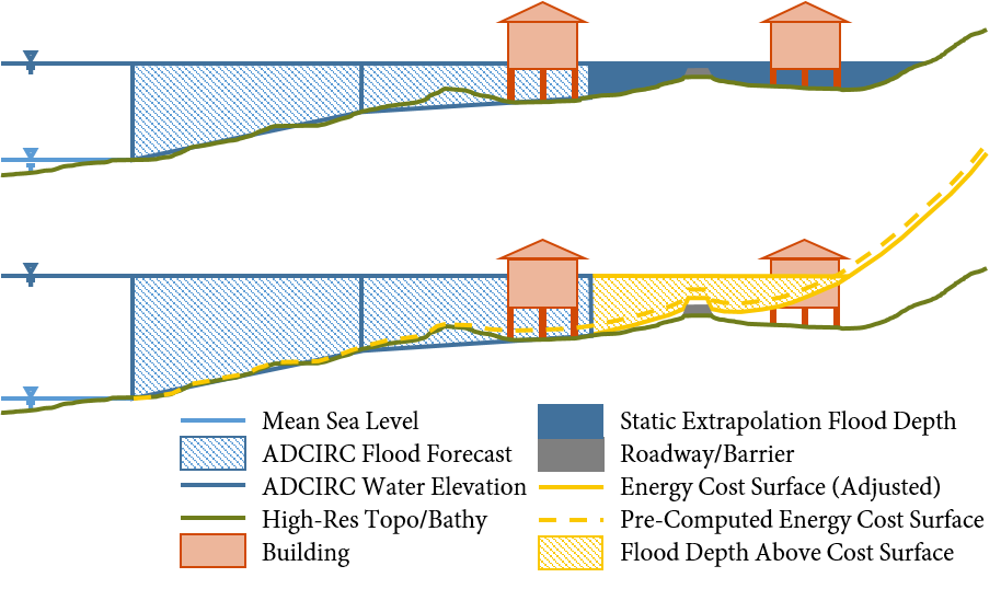
Side-view schematic of downscaling methods. A one-dimensional schematic is displayed for each of the two downscaling methods, where the top figure is the static method and the bottom is the head loss method. In the static method, the water elevations from ADCIRC (blue hatched portion) are extrapolated as a flat surface until they intersect the DEM. In the head loss method, these water elevations are extrapolated to an energy cost surface (elevation plus cumulative head loss).

Theory

The head loss method was developed to improve the accuracy of downscaling. In the static method, the only way to stop water from increasing its lateral extent is for the surface to reach a barrier or topographical surface represented by the DEM or to reach a maximum extrapolation radius. In reality, as water floods over a surface, energy is dissipated as it comes into contact with any form of roughness that might interfere with the flow. This causes flooding extents to be limited based on the magnitude of energy loss due to friction. Overland flow caused by storm surge is hindered most by hard structures and dense vegetation, while developed surfaces and wooded wetlands allow the surge to flow more freely (although energy is still being dissipated). This is a common hydraulic principle and is included in many numerical models, including ADCIRC.

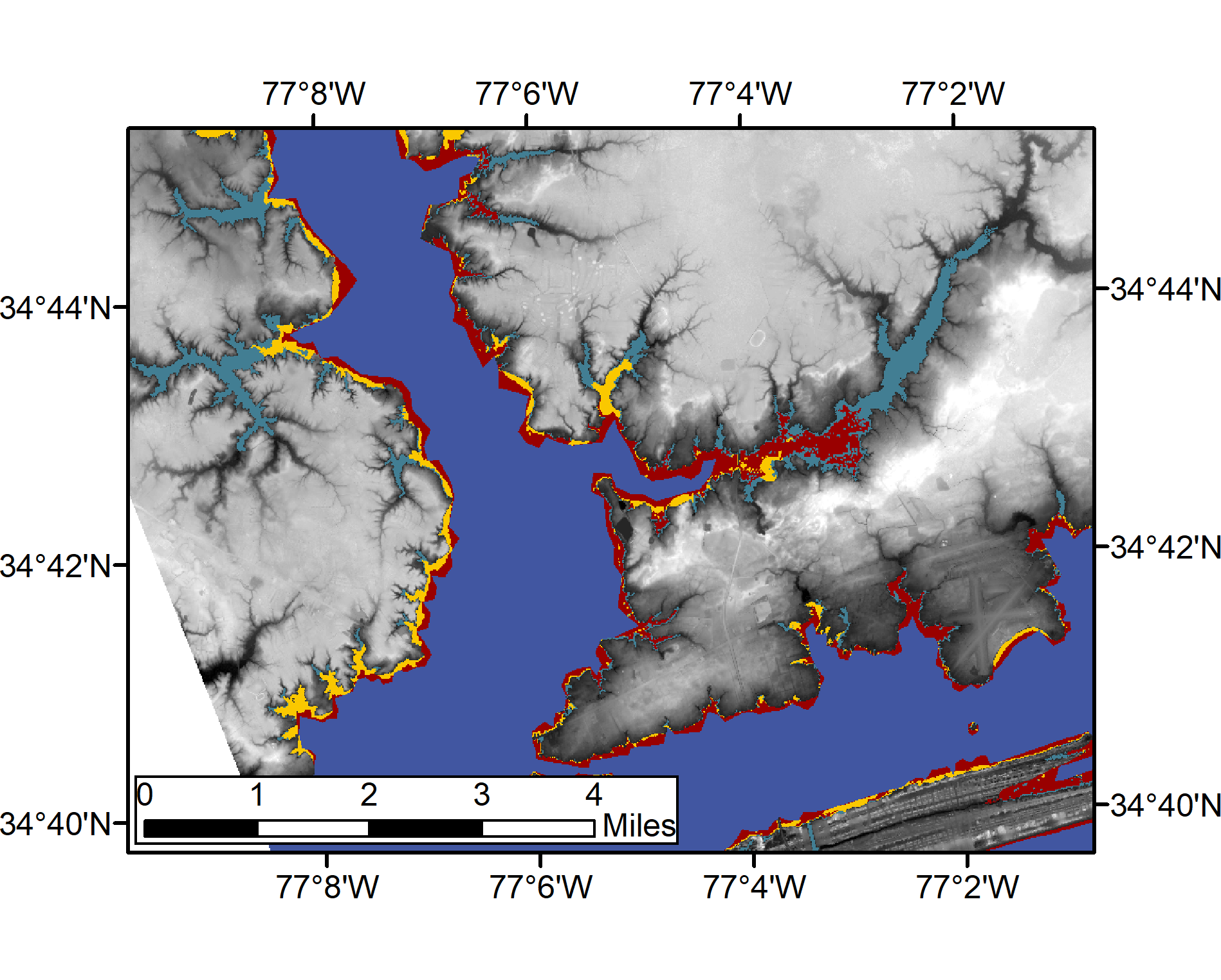
Comparison of flood extent results. Results are displayed in plan view, showing the differences in flood extents for each downscaling method. ADCIRC water elevations from a simulation using the NC9 mesh (indigo, top layer) were downscaled using the head loss method (yellow) and the static method (blue). These are compared to a high-resolution ADCIRC simulation (red), which is considered as truth. More information about the accuracy of each downscaling method can be found in the thesis Rucker 2020.

The head loss method operates similarly to the static method in that water elevations are extrapolated horizontally until intersecting a raster surface. The major difference is, instead of using a DEM as this raster surface, the head loss method uses an “energy cost” surface. This cost surface represents the elevation added to the total accumulation of head loss occurring as water travels from MSL to each point in the raster.

To create a cost surface, the user must first create a GRASS location using a selected DEM, as discussed in the aforementioned web page. The user must then provide a raster containing land cover classifications throughout the region covered by the DEM. A good source for land cover classification data in the U.S. is the USGS National Land Cover Database (NLCD). A raster (30 m resolution) containing the most recent data can be downloaded using this link.

Land cover classifications can be directly associated with friction coefficients by assigning a Manning’s $n$ coefficient to each classification. This is a common research topic, and there is a range of acceptable $n$ values for each classification. The GitHub page for Kalpana contains a file called landCover_manning.txt with recommended values for each NLCD classification based on literature (Liu et al. [2018], Kalyanapu [2009]). To use different classification numbers or Manning’s $n$ values, follow the format shown in landCover_manning.txt, where the value on the left is the number associated with each land cover type, and the value on the right is Manning’s $n$ multiplied by 10,000.

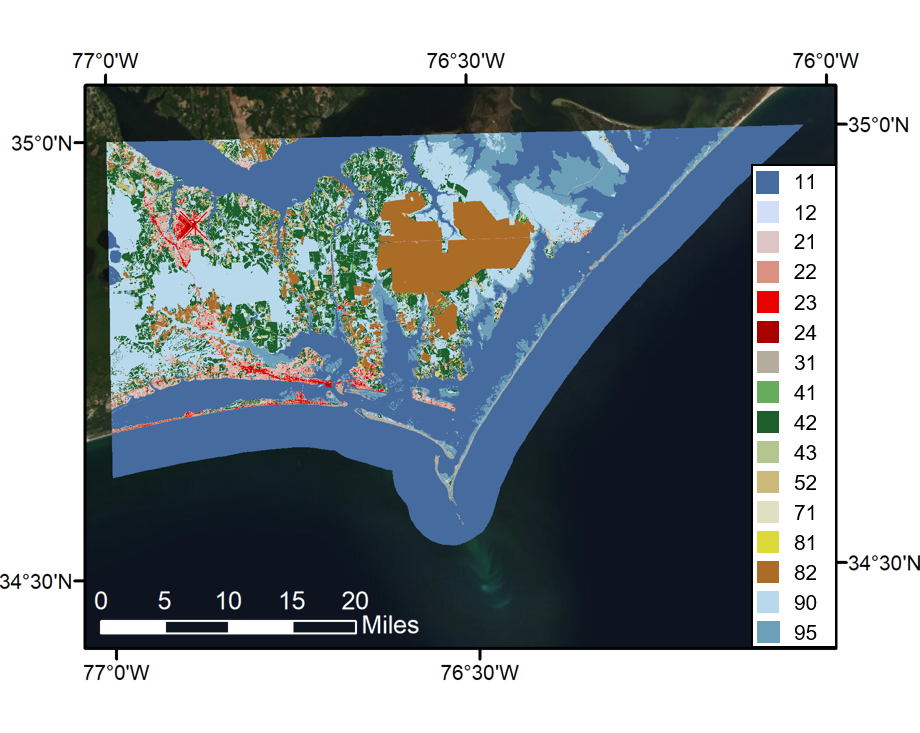
NLCD raster. The land cover raster used in Example A is shown, where each land cover type is assigned a color and number, as shown in the legend.

The head loss method uses Manning’s equation to calculate head loss as overland flooding occurs. Manning’s equation is typically used for channel flow, but can be used in overland flow by assuming a wide channel, where hydraulic radius becomes approximately equal to the depth of flow. Manning’s equation is:

(1) $\begin{equation*} U = \frac{ k }{ n } R^{2/3} S^{1/2} \end{equation*}$

where $U$ is the flow velocity, $k$ is a unit conversion factor ( $k=1$ for SI units; $k=1.49$ for U.S. customary units), $n$ is Manning’s coefficient, $R$ is the hydraulic radius, and $S$ is the slope of the energy grade line. The slope of the energy grade line can be interpreted as the friction slope $h_L$ , where $h_L$ is head loss and $L$ is the lateral distance traveled. By manipulating Manning’s equation, head loss can be calculated directly:

(2) $\begin{equation*} h_L = L \left( \frac{ n U }{ k R^{2/3} } \right)^2 \end{equation*}$

in which $L$ represents the distance between the center of each raster cell and $h_L$ represents the vertical reduction in water surface elevation over distance $L$ .

Adding cumulative head loss to the DEM (potential energy) creates the form of total energy cost required to travel from MSL to any point in the raster. The total cost is calculated as:

(3) $\begin{equation*} \text{cost}_\text{total} = \Delta z + \sum L \left( \frac{ n U }{ k R^{2/3} } \right)^2 \end{equation*}$

where $\Delta z$ is the change in elevation represented by the DEM and the second right-hand-side term is the total accumulation of head loss over flow paths from MSL to a given point.

To maximize efficiency in forecasting, the head loss method computes the energy cost surface prior to receiving input from ADCIRC. Two issues arise from this process: (1) prior to receiving input from ADCIRC, the hydraulic radius and velocity are unknown at each raster cell, and (2) the flow paths over which the accumulation of head loss occurs are unknown. To overcome these issues, the energy cost surface is computed using synthetic values for $U$ and $R$ with the r.walk GRASS GIS module. This process is described further in the master’s thesis by Carter Rucker [2020].

The synthetic values for $U$ and $R$ during the pre-computational phase are lumped into one constant that is used throughout the domain. This constant is referred to as $UR_\text{const}$ and represents $U/R^{2/3}$ . The constant will be set to the default value of 1 unless changed using the --urconst option. Increasing $UR_{const}$ will increase the effect of friction in determining flow paths, while decreasing the constant will increase the effect of elevation changes for the flow paths.

The r.walk GRASS module computes the cumulative energy cost required to travel from MSL to one specific endpoint. All points from MSL are finding the “least cost paths”, or paths requiring the least amount of energy, to travel to the selected endpoint; changing this endpoint would alter the least cost paths generated. Therefore, to create an energy cost raster for the whole domain, multiple endpoints for r.walk must be used. Operating r.walk with endpoints for each raster cell above MSL would be redundant, so instead this is done for an array of endpoints.

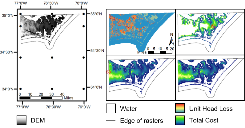
Iterative cost surface generation. The cost surface is created by executing r.walk to calculate the least amount of energy required to travel from MSL towards each endpoint and keeping the lowest cost value from all iterations at each raster cell. The 12 endpoints for each r.walk iteration used in the example problem below are shown as black dots on the left image. The top middle is the unit head loss raster, which is directly related to each raster cell’s Manning’s n coefficient. The top right and bottom middle images show resulting rasters from two different iterations, in which the encircled red X represents the endpoint. The raw cost raster is shown on the bottom right.

The density of this array is controlled using the --numcols option, which specifies the number of columns spanning from the left edge of the domain to the right edge. The spacing of these columns will also be used as the spacing between rows. The default value for --numcols is 5 so, if this default value is used and the domain is slightly taller than it is wide, the array will have 6 rows; a row is automatically placed along the top and bottom edges of the domain.

Example Using --createcostsurface yes

To create a cost surface for use with the head loss method, the current working directory must contain all of the necessary files. First, a GRASS location must be created by following instructions from Example 1 on the page Downscaling ADCIRC Flooding Inundation Extents Using Kalpana, using the specified DEM. This will create the file GRASS_LOCATION.zip, which is the GRASS location used for the static method and only contains the DEM raster and associated projection information. The working directory must also contain kalpana.py, GRASS_LOCATION_wgs84.zip, and landCover_manning.txt, which can all be downloaded from the GitHub website for Kalpana.

Finally, it is recommended for the user to provide a land classification raster using the --landcoverraster option. By default (or by specifying --landcoverraster NLCD2016), Kalpana will try to download the NLCD 2016 raster for the entire contiguous U.S., then clip the raster based on the extents of the provided DEM. However, depending on the Internet permissions and settings, this default process may fail, so this example uses a small raster that covers the extents of the DEM.

Example A: Create an Energy Cost Surface

First, download the necessary files kalpana.py, oneTileNLCD.tiff, GRASS_LOCATION_wgs84.zip, and landCover_manning.txt from the GitHub page for Kalpana.

Then, download the DEM n35w077 and follow Example 1 from Downscaling ADCIRC Flooding Inundation Extents Using Kalpana to create GRASS_LOCATION.zip.

Finally, run the line of code below to execute the pre-computational process for creating an energy cost surface, which uses the default value for --urconst and a value less than the default for --numcols. A smaller number of columns was chosen to reduce computation time.

python ./kalpana.py --createcostsurface yes --landcoverraster "oneTileNLCD.tiff" --numcols 3 --urconst 1

This process will create an array with 12 r.walk endpoints and should complete in about 25 minutes. After completion, this will leave a file called HEADLOSS_LOCATION.zip that contains the DEM and a raster called rawCost. The rawCost raster is simply the total energy cost, stripped of the DEM and $UR_{const}$ .

(4) $\begin{equation*} \text{cost}_\text{raw} = \sum L \left( \frac{ n }{ k } \right)^2 \end{equation*}$

In the later examples, after receiving input from ADCIRC, this raster will be populated with actual values, rather than the synthetic $UR_\text{const}$ values and added to the DEM to create the total energy cost surface. The working directory is now prepared to downscale ADCIRC water elevations using the head loss method.

Examples Using --grow headloss

After receiving maximum water elevations from ADCIRC, these values can be used to compute the cost surface and downscale water elevations. To compute the cost surface, $U$ and $R$ values must be used with the raw cost raster to fill in the missing portions of the total cost. $R$ is calculated as the average depth between MSL and each raster point of interest ( $R_\text{avg}$ ). These depths are based on the difference between the water elevation from static extrapolation and the DEM elevation.

The ADCIRC wetting and drying algorithm only allows elements to be wet or dry. Therefore, at the edge of the ADCIRC output, water velocities ( $U$ ) are low and unreliable for extrapolation. Instead of using these values, a constant value is used for $U$ throughout the domain. Using a constant value also saves computational time with minimal effect on results. A constant friction exaggeration value can be implemented using the --fricexagval option. This is similar to changing the constant $U$ value because each has an effect on the head loss throughout the domain. Increasing --fricexagval will increase the amount of head loss, thus decreasing the flood extent, and vice versa.

The raw cost raster is multiplied by $(U/R_\text{avg})^2$ to create a raster filled with head loss values for each raster cell. This raster is added to the DEM to create a total cost surface. Finally, the water elevations are extrapolated to the cost surface and elevations greater than the energy cost are kept in the final water elevation raster.

This page will work through two examples for downscaling with the head loss method. These examples will require the user’s working directory to contain kalpana.py, HEADLOSS_LOCATION.zip, GRASS_LOCATION_wgs84.zip, and maxele.63.nc.

Example B: Create Output for Downscaled Water Elevations in Shapefile Format

The following line of code will create a shapefile binned by similar water elevations based on the --contourrange option. Required input options include --storm, --filetype, --contourrange, --units, and --grow. Optional input options include --flooddepth, --grownoutput, and --fricexagval.

python ./kalpana.py --storm florence --filetype maxele.63.nc --contourrange "0 21 0.5" --units english --grow headloss --flooddepth no --grownoutput headloss_downscaled_shp --fricexagval 1

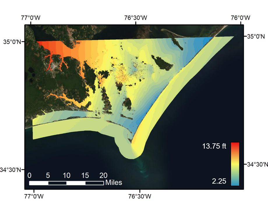
Water elevations, downscaled using the head loss method, are shown in polygon shapefile format. Water elevations are binned in groups of 0.5 ft, with the value set to the average of each bin.

Example C: Create Output for Downscaled Water Depths in Raster Format

The following line of code will create a raster of water depths (--flooddepth yes), which are represented by the water elevation minus the DEM elevation. Required and optional input options are the same as in the previous example.

python ./kalpana.py --storm florence --filetype maxele.63.nc --contourrange "0 21 0.5" --units english --grow headloss --flooddepth yes --grownoutput headloss_donwscaled_depths --fricexagval 1

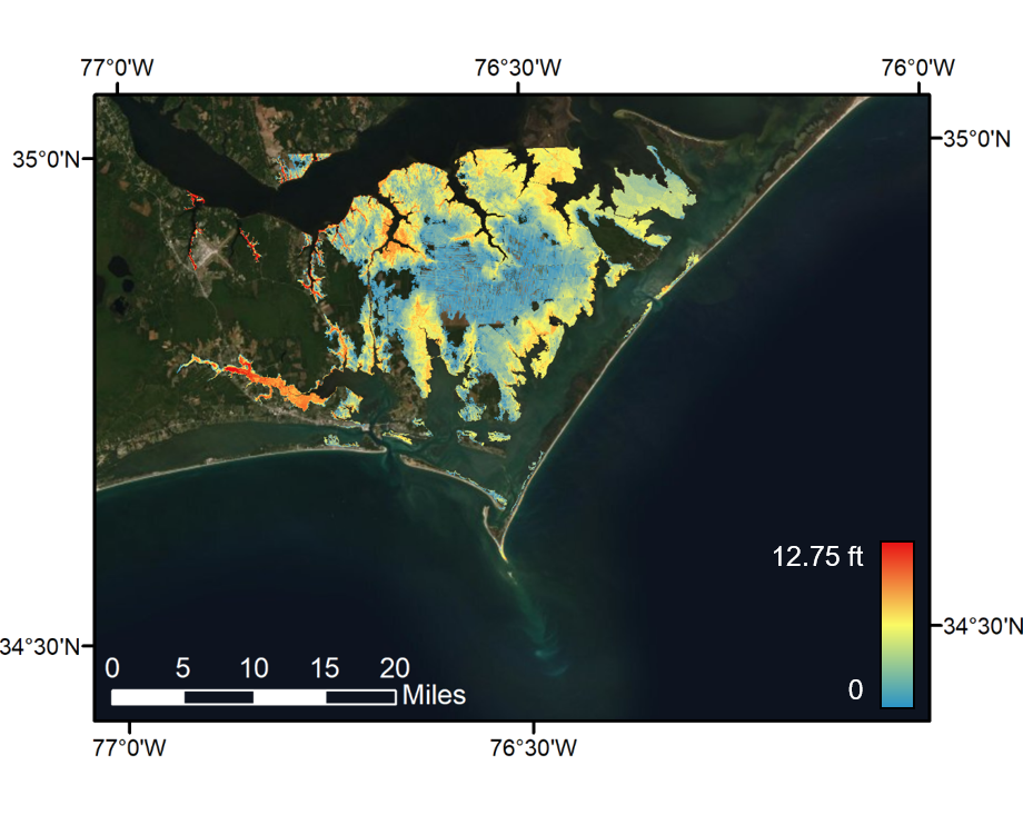
Flood depths of downscaling results using the head loss method are displayed in raster format.

Summary of Kalpana Options for Head Loss Method

Table 1: Create Cost Options

Option Added	Choices	Purpose/Usage:
`createcostsurface`	`yes`, `no`; default=`no`	Choose `yes` to create a GRASS location with a DEM and a raster cost surface. This location must exist to downscale water elevations using the head loss method (`--grow headloss`). The location created will be called HEADLOSS_LOCATION.zip and will contain the DEM and the raw cost raster.
`landcoverraster`	“`[string]`”; default=”`NLCD2016`“	Specify the name of the raster containing land cover classification data using a relative path. By default, Kalpana will automatically download the land classification raster from NLCD for 2016, which covers the entire U.S. This is not recommended, as the this would be time-consuming and may fail, depending on the system’s Internet permissions.
`numcols`	`[integer]`; default=`5`	Select the number of columns in the array of `r.walk` endpoints. Columns will automatically be made on the left and right edges of the domain. The same spacing between columns will be used as the spacing between rows, with rows placed at the top and bottom of the domain. Therefore, if a domain is taller than it is wide, there will be more rows than columns.
`urconst`	`[float]`; default=`1.0`	Set a value for $UR_{const}$ . Higher values will add more emphasis on friction in determining flow paths, while lower values will add more emphasis on elevation in determining flow paths.
“landCover_manning.txt”	default=given file	Define the Manning’s $n$ values for each classification in the land cover raster. The given file contains values corresponding with the NLCD raster, based on literature. If other values are desired use the syntax shown in the provided “landCover_manning.txt” file, where [classification number]=[Manning’s $n$ * 10,000].

Table 2: Options for Downscaling

Option Added	Choices	Purpose/Usage
`grow`	`static`, `headloss`, `yes`, or `no`; default=`no`	Select `headloss` to downscale using the head loss method. To accommodate for older versions of Kalpana, selecting `yes` will execute the static method.
`fricexagval`	`[float]`; default=`1.0`	Universally scale the friction values throughout the domain. Increasing the friction will universally reduce the flood extents after downscaling; the opposite will occur if friction is decreased.

References

Kalyanapu, A et al. (2009). “Effect of land use-based surface roughness on hydrologic model output.” Journal of Spatial Hydrology 9.2, pp. 51-71.

Liu, Z et al. (2018). “Investigating the role of model structure and surface roughness in generating flood inundation extents using one- and two-dimensional hydraulic models.” Flood Risk Management 12.1, pp. 1-19.

Rucker, C (2020). “Improving the Accuracy of a Real-Time ADCIRC Storm Surge Downscaling Model.” Master’s thesis. Raleigh, NC, USA: North Carolina State University.