
Updated 2020/06/24: Added documentation for --growradius none option.
Updated 2020/04/15: Added documentation for DEM vertical unit conversions.
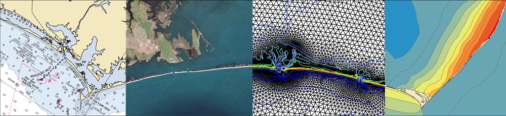
The ADCIRC modeling system is used often to predict coastal flooding due to tropical cyclones and other storms. The model uses high resolution to represent the coastal environment, including flow pathways (inlets, man-made channels, rivers) and hydraulic controls (barrier islands, raised features). However, due to the use of large domains to represent hazards on coastlines in an entire state or multiple states, the highest resolution is typically about 20 to 50 m in coastal regions. Thus, there is a potential gap between the flooding predictions and the true flooding extents. We have developed a geospatial software to downscale the flooding extents to higher resolution.
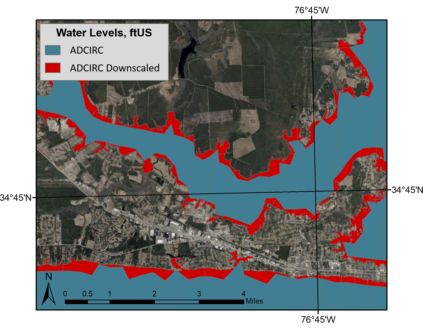
ADCIRC vs. downscaled water levels, plan view. This image shows the difference in prediction of flooding extents, with the blue portion representing the original ADCIRC flooding extents and red representing the downscaled extents.
The following documentation is for downscaling the flooding predictions by using Kalpana. This software was created originally to view ADCIRC outputs as either ESRI shapefiles or KML files (for viewing in Google Earth). ADCIRC (the ADvanced CIRCulation model) uses finite element methods to predict water levels throughout the modeled domain. Although this model is able to provide accurate predictions in a matter of minutes, these predictions have a limited resolution and are not able to provide information at the scale of buildings, roadways, and other critical infrastructure.
This addition to Kalpana is able to predict water levels and flooding extents at the scale of critical infrastructure by downscaling water levels to a DEM (digital elevation model) with a finer resolution. To achieve this, Kalpana uses GRASS GIS and a DEM chosen by the user to horizontally extrapolate the ADCIRC predicted water elevations until an equivalent or greater DEM elevation is reached (shown in the figure below). The primary operation executed in this code for extrapolation is a GRASS module called r.grow, where “r” indicates a raster operation. Therefore any allusion to growth in this documentation such as “r.grow” or “--grow" is referring to the water level downscaling process.
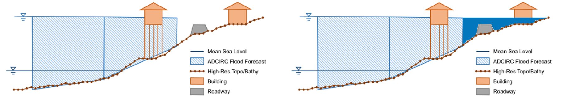
Water level downscaling illustration in profile view. The image on the left represents the ADCIRC water levels, while the image on the right shows the additional downscaled water level extents via horizontal extrapolation.
In order to execute the r.grow extrapolation process, a GRASS location must first be created using the --createlocation option and a DEM of choice. A GRASS location is required for any operations done in GRASS GIS because it contains all of the necessary data (rasters, vectors, etc.) as well as the appropriate datum information for the given data. A great place to download DEMs in the United States is USGS TNM: https://viewer.nationalmap.gov/basic/. If using this website, it is recommended to download elevation products (3DEP) with 1/3 arc-second resolutions; this option is available for the entire United States.
Any DEMs used to create a GRASS location must use a datum with state plane coordinates because the code cannot be executed properly if units are in degrees (lon/lat). If the user is certain the DEM uses state plane coordinates and contains the desired resolution, specify --createmethod existing (shown below) to create a GRASS location based on the existing datum of the DEM. If unsure whether the DEM uses the correct datum or the DEM does not use the correct datum, use the --epsg option to automatically convert the data to a correct state plane coordinate system of choice. The correct EPSG code varies depending on region (typically different state-to-state in the US) and can be found using the following website: http://spatialreference.org/ref/.
Important Notes to Remember
- Kalpana is currently hard-wired to call GRASS GIS version 7.2. If using a different version, search the kalpana.py document and replace grass72 with the appropriate grassXX version (e.g. if using GRASS GIS version 7.6, change every grass72 to grass76). Keeping this hard-wired allows users to only need to make this change once, rather than entering this option for every run.
- Remember that these flood elevation outputs (unless using the
--flooddepthoption) are relative to mean sea level (MSL), not mean water level (MWL). Therefore, if the user is interested in data further upstream away from the ocean, the mean water level may be greater than 0. Remember this when setting the minimum and maximum contour levels. - As a reminder, the latest version of Kalpana (along with the necessary WGS84 GRASS location) can be downloaded from https://github.com/ccht-ncsu/Kalpana.
- The Kalpana code is currently only executable in Linux systems; this code will not work if executed in a Windows or Mac OS environment.
- The
--contourrangeoption only controls the contour range for use with the original version of Kalpana. As of now, shapefiles created using the--growoption will contain binning of 0.5 feet (or meters).
Below are examples of correctly used --createlocation options. To mimic these examples, download the following two DEM rasters from USGS TNM:
- USGS NED 1/3 arc-second n35w077 1 x 1 degree ArcGrid 2015
- Product ID: 581d213ee4b08da350d52e09
- Download dem_n35w077
- USGS NED 1/3 arc-second n35w078 1 x 1 degree ArcGrid 2015
- Product ID: 581d213ee4b08da350d52e02
- Download dem_n35w078
For these examples, all accompanying files included in each zip folder can be erased other than the folders containing each DEM (folders grdn35w077_13 and grdn35w078_13).
These two DEMs were chosen to use in Kalpana examples for multiple reasons. First, during construction of the r.grow extrapolation code, testing was hard-wired to a North Carolina DEM, and the code was later manipulated to accommodate for any location. Therefore, the two chosen DEMs (located within and around Cape Lookout, NC) are well-tested and will provide accurate results. Second, USGS 1/3 arc-second (approximately 30 ft) resolution DEMs are chosen because this type of DEM is accessible to the public, and USGS provides coverage for 1/3 arc-second data throughout the entire United States. Last, since these DEMs do not contain the correct datum for use with r.grow, this allows the user to practice choosing a correct EPSG code to convert to the correct datum. These DEMs use a datum which contains units of latitude and longitude, rather than state plane coordinates (feet or meters). Additionally, the DEMs use vertical units of meters, but the examples use water elevations in feet. This requires the user to utilize an option that automatically converts vertical units from meters to feet.
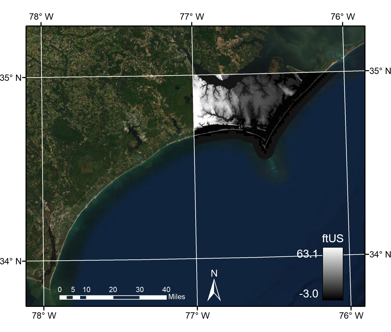
For reference, the full patched DEM (including both the n35w077 and n35w078 DEMs) is pictured below:
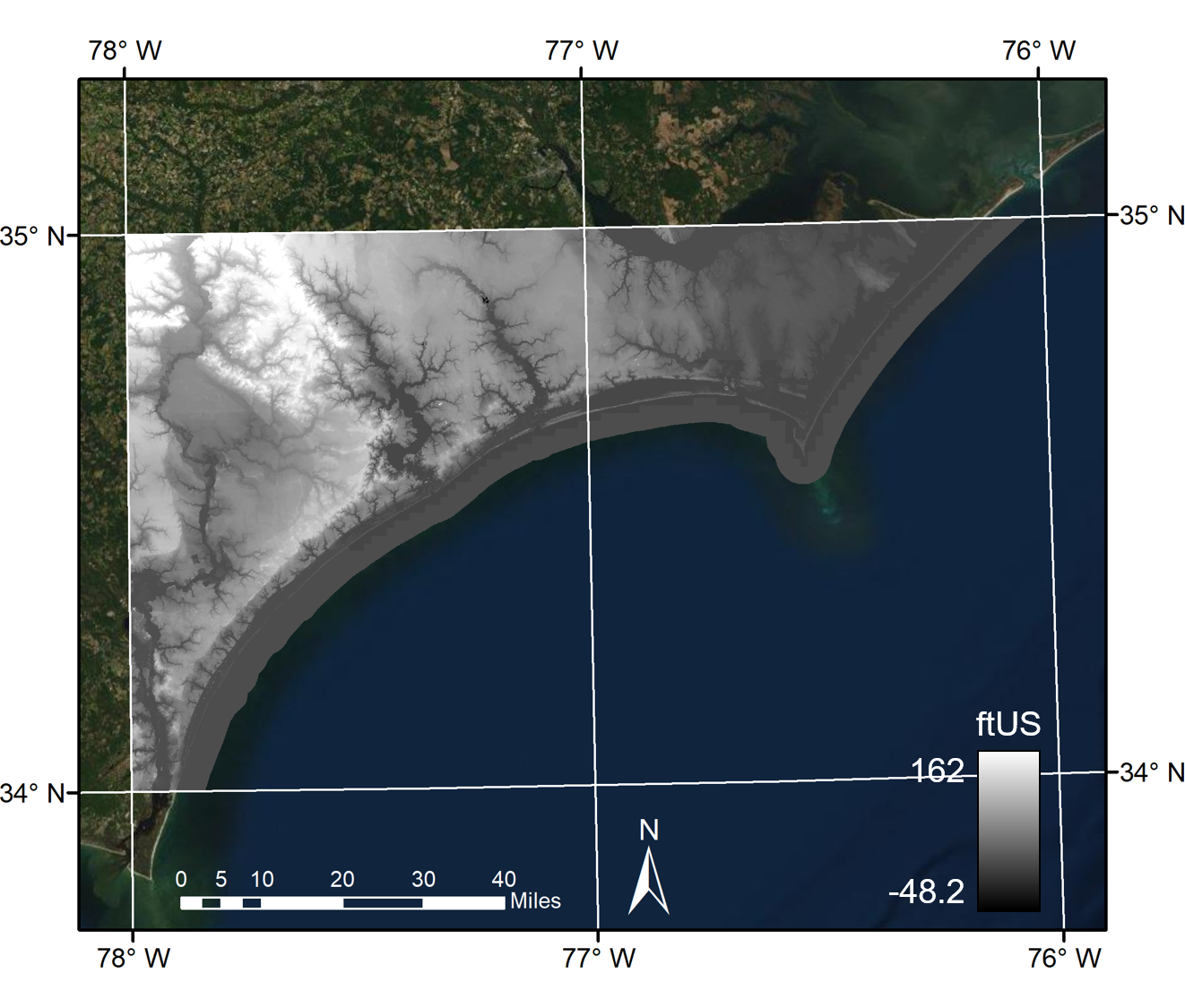
Full DEM raster created by patching the n35w077 and n35w078 rasters.
Examples Using --createlocation yes
Before starting with these examples, make sure the current working directory contains all of the necessary files. The current working directory should contain kalpana.py, the two folders containing raster data (grdn35w077_13 and grdn35w078_13), and a job script (if desired). Further explanations for each of the available options are provided in table 1 below. Each example includes a vertical unit conversion of meters to feet using the --vunitconv option.
Example 1: Specified resolution and EPSG code.
Create a location using one raster with a specified resolution of 50 ft and a specified EPSG code of 2264. Estimated time required for completion: 90 seconds.
python ./kalpana.py --createlocation yes --raster "./grdn35w077_13/w001001.adf" --resolution 50 --epsg 2264 --vunitconv m2ft
Single n35w077 DEM raster. This DEM is used for examples 1-3, while examples 4-6 use the full patched raster shown in the previous figure.
Example 2: Keep original raster resolution and use specified EPSG code.
Create allocation using one raster, keeping the raster’s original resolution, and using a specified EPSG code of 2264. This example requires about 180 seconds to complete using the example rasters, because these rasters use a resolution finer than 50 ft.
python ./kalpana.py --createlocation yes --raster "./grdn35w077_13/w001001.adf" --resolution align --epsg 2264 --vunitconv m2ft
Example 3. Keep original raster resolution and datum.
Create a location using one raster, keeping its original datum and resolution. This method only requires about 10 seconds for completion, but should be used with caution. As seen in this example, the input raster contains data in latitude and longitude, making it unable to be used with r.grow if --createmethod existing is specified.
python ./kalpana.py --createlocation yes --raster "./grdn35w077_13/w001001.adf" --createmethod existing --vunitconv m2ft
Example 4: Specified resolution and EPSG code using multiple rasters.
Create a location using two rasters with a specified resolution of 50 ft and a specified EPSG code of 2264. Estimated time required for completion: 200 seconds.
python ./kalpana.py --createlocation yes --raster "./grdn35w077_13/w001001.adf,./grdn35w078_13/w001001.adf" --resolution 50 --epsg 2264 --vunitconv m2ft
Example 5: Keep original raster resolution and use specified EPSG code using multiple rasters.
Create a location using two rasters, keeping the rasters’ original resolution, and using a specified EPSG code of 2264. When using multiple rasters with the align option, the resolution used is equal to the first listed resolution. This example requires about 380 seconds to complete using the example rasters because these rasters use a resolution finer than 50 ft and multiple rasters are being used.
python ./kalpana.py --createlocation yes --raster "./grdn35w077_13/w001001.adf,./grdn35w078_13/w001001.adf" --resolution align --epsg 2264 --vunitconv m2ft
Example 6: Keep original raster resolution and datum using multiple rasters.
Create a location using two rasters, keeping the original datum and resolution. This option also uses the resolution and datum of the first listed raster. This method only requires about 60 seconds for completion, but should be used with caution. As seen in this example, the input raster contains data in latitude and longitude, making it unable to be used with r.grow if --createmethod existing is specified.
python ./kalpana.py --createlocation yes --raster "./grdn35w077_13/w001001.adf,./grdn35w078_13/w001001.adf" --createmethod existing --vunitconv m2ft
After --createlocation is executed, there will be a file called GRASS_LOCATION.zip in the current working directory. To execute r.grow, the current working directory must contain GRASS_LOCATION.zip, GRASS_LOCATION_wgs84.zip, kalpana.py, and the appropriate maxele.63.nc file. The --grow option has required inputs of: --storm (enter the storm name), --filetype (typically maxele.63.nc), --contourrange (“[min] [max] [step]”), and --units (english or metric) with optional inputs including: --grownoutput, --growmethod, --growradius, --flooddepth, and --grownfiletype (all documented in table 2 below).
Examples Using --grow yes
Before starting with these examples, make sure the current working directory contains all of the necessary files. The current working directory should contain kalpana.py, GRASS_LOCATION.zip (created using --createlocation), maxele.63.nc (or other filetype), GRASS_LOCATION_wgs84.zip (which can be downloaded from the GitHub portal), and a job script (if desired). The following examples all use the GRASS location created in Example 1, using only the n35w077 raster with a specified resolution of 50 ft and a specified EPSG code of 2264. Each example requires about 90 seconds for completion.
A sample maxele.63.nc file can be downloaded and unzipped using this link. This file contains ADCIRC outputs for the maximum water levels occurring throughout the duration of advisory 48 of Hurricane Florence (2018) using a segmented portion of an HSOFS (Hurricane Surge On-Demand Forecast System) mesh. This mesh was developed by NOAA for use in the NSEM (Named Storm Event Model) to make storm predictions throughout the eastern portion of the United States. Advisory 48 was one of the more severe advisories for coastal North Carolina, so users are able to visualize more extreme water levels and further r.grow extrapolation extents. Further explanations for each of the r.grow options are provided in Table 2 below.
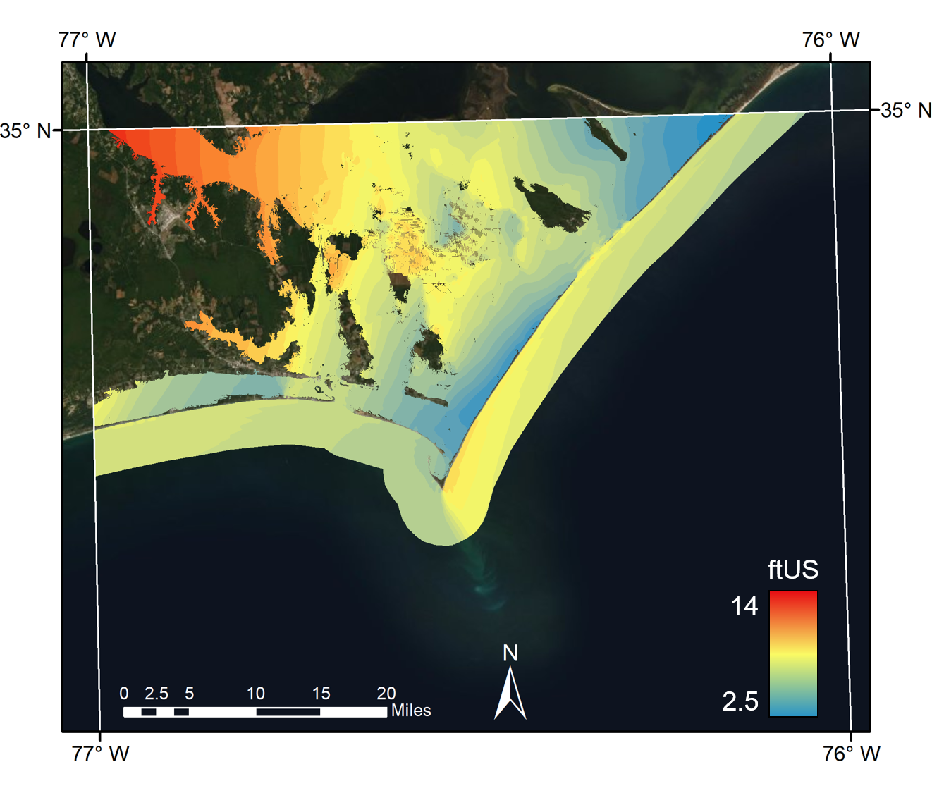
Example 7: Grow using default inputs.
Operate r.grow using the required inputs (--storm, --filetype, --contourrange, --units) as well as the default settings for the optional inputs (--grownoutput, --growmethod, --growradius, --floddepth, --grownfiletype). As shown in the subsequent examples, since these optional inputs are all set to their default values in the current example, leaving out these options will result in the same operation.
python ./kalpana.py --storm florence --filetype maxele.63.nc --contourrange "0 21 0.5" --units english --grow yes --grownoutput WaterLevels_grownDefaults --growmethod without --growradius 30.01 --flooddepth no --grownfiletype ESRI_Shapefile

Downscaled water levels using default values.
Example 8: Grow using the subtraction method.
Operate r.grow using the subtraction method (--growmethod with), with all other optional values set to default. Using the subtraction method removes raster cells from the original ADCIRC predictions where the water level is lower than the corresponding ground surface elevation before the r.grow extrapolation step occurs.
python ./kalpana.py --storm florence --filetype maxele.63.nc --contourrange "0 21 0.5" --units english --grow yes --grownoutput WaterLevels_grownWith --growmethod with
Downscaled water levels using the subtraciton method. Only subtle differences can be seen in comparison to the defaults example for this particular storm advisory.
Example 9: Grow using an increased radius.
Operate r.grow using an increased radius of 60 cells, with all other optional values set to default. The radius is used to limit the extent of growth due to horizontal extrapolation where the water is not fully stopped by the DEM elevation. The radius is in units of cells, so for instance a radius of 30 with a raster cell resolution of 50 ft will allow for a maximum horizontal growth of 1500 ft away from the original ADCIRC water levels. The grow radius check can be bypassed by using the option --growradius none. This will reduce computational time, but the maximum extents of extrapolation will only be limited by the DEM. The recommended radius value for North Carolina is set to the default, 30.01.
python ./kalpana.py --storm florence --filetype maxele.63.nc --contourrange "0 21 0.5" --units english --grow yes --grownoutput WaterLevels_grown60 --growradius 60.01

Downscaled water levels using an increased grow radius of 60.01. Notice that this example is grown further horizontally in some areas as compared to the previous two examples.
Example 10: Visualize grown results as flood depths.
Operate r.grow and visualize results as flood inundation depths, rather than flood elevations, with all other optional values set to default. This option simply takes all of the flood elevations covering any terrestrial DEM areas and subtracts the DEM value, resulting in flood depth. These data are visualized as a raster rather than polygons because, even if binning occurs, there are still too many unique polygons. This will cause creating and exporting a polygon to actually take longer than just exporting a raster.
python ./kalpana.py --storm florence --filetype maxele.63.nc --contourrange "0 21 0.5" --units english --grow yes --grownoutput FloodDepth --flooddepth yes
NOTE: GRASS GIS sometimes has issues exporting the color table of this image, creating an error message and causing the output TIFF to contain outliers which throw off the coloring. A simple solution to this issue is to perform a raster calculation using the Raster Calculator in ArcMap. An example equation could be:
Con(("floodDepths.tif">0)&("floodDepths.tif"<50),"floodDepths.tif").
This will remove all values below 0 ft and above 50 ft elevation and set the color table to the remaining minimum and maximum raster values.
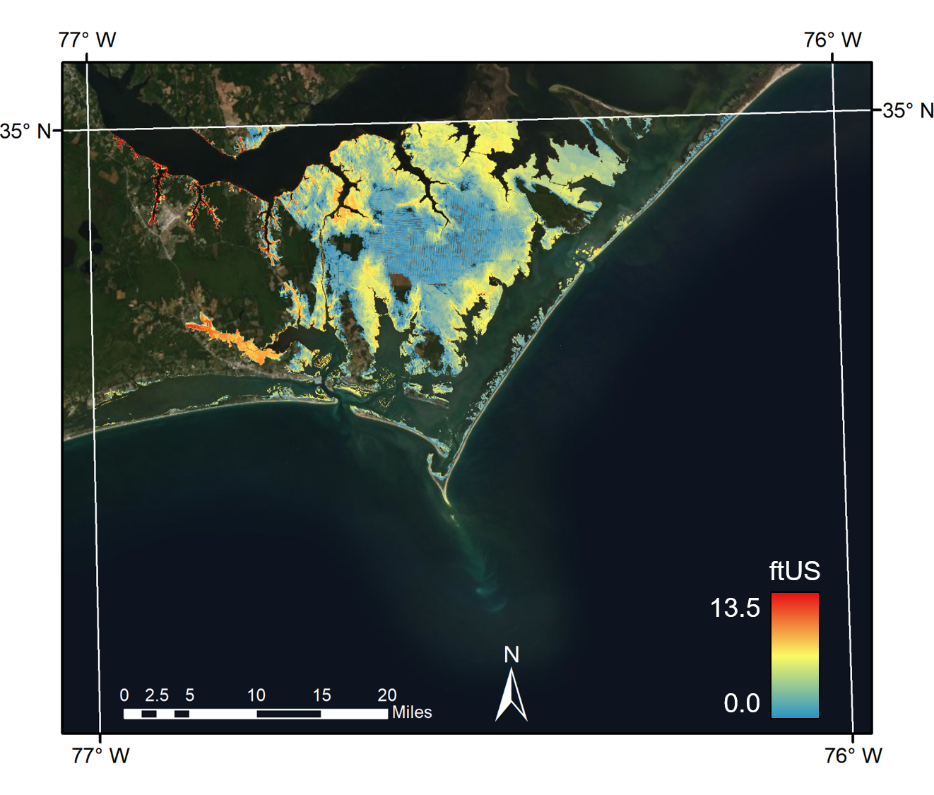
Inundated flood depths example. These values are generated by subtracting the DEM elevation from the water elevation in areas where the DEM has a value greater than zero (i.e. sub-aerial DEM only).
Example 11: Visualize grown results in KML format.
Operate r.grow and visualize flood elevations as KML by changing –grownfiletype, with all other optional values set to default.
python ./kalpana.py --storm florence --filetype maxele.63.nc --contourrange "0 21 0.5" --units english --grow yes --grownoutput WaterLevels_grownKML --grownfiletype KML
Table 1: Create Location Options
| Option Added | Choices | Purpose/Usage: |
|---|---|---|
| createlocation | yes, no; default=no |
Switching to yes will automatically create a GRASS location (
GRASS_LOCATION.zip) for use with r.grow extrapolation. This location file must exist before executing r.grow (--grow yes). createlocation requires arguments for raster and either --epsg (if the user wishes to create a GRASS location by defining the EPSG state plane coordinate system) or --method existing. method existing must only be used if the user is certain that the input DEM uses a state plane coordinate datum and contains the desired raster resolution. Otherwise, the location should be created using the EPSG method. |
| raster | “[string]” |
If only one DEM raster is to be used, input the name of the raster as a string (including quotation marks) and save the raster to either the current folder or its own separate folder containing all of the necessary accompanying raster files (e.g.
“./rasterFolder/myRaster.adf”). If multiple rasters are to be used, it is recommended to save each raster into a separate folder within the current working directory and enter their paths as a comma-delimited string (e.g. “./rasterFolder1/myRaster1.adf,./rasterFolder2/myRaster2.adf”).NOTE: Some formats (such as .adf) require accompanying files. For instance, DEMs downloaded from the USGS TNM database require both the w001001.adf (the raster itself) and its accompanying files to be present in the current working directory (for one raster) or in its respective folder (for multiple rasters). However, only the w001001.adf file needs to be specified with the --raster option. |
| resolution | [number], align; default=50 |
Setting the resolution to a number specifies both the GRASS location and DEM resolutions, using units set by the GRASS location. For example, a GRASS location created using EPSG 2264 for NAD83/North Carolina (ftUS) with resolution set to 100 will force the resolution to become 100 ft. Setting the resolution to align will allow both the GRASS location and the DEM to keep the resolution of the input DEM. WARNING: if multiple DEMs are used, the align feature will use the resolution of the first raster listed.
|
| epsg | [integer] |
Specify the EPSG code to be used for creating the GRASS location. The selected projection must use linear distance units (i.e. NOT latitude/longitude). If the necessary EPSG code is unknown, the correct code can be found using the following link: http://spatialreference.org/ref/?page=7&search. If this is not used with
--createlocation, please set --method to existing to use the datum of the existing raster (described below). |
| createmethod | existing; default=null |
If this option is set to
existing, the GRASS location will be generated using an existing DEM, as specified by the --raster input. This can only be done for one raster and only if the user is certain that the raster uses the correct projection (using linear distance units of feet or meters and not latitude/longitude) and the raster contains the desired resolution. If this option is not used with --createlocation, the user must specify the --epsg option. |
| vunitconv | m2ft, ft2m; default=no |
If the vertical units of the DEM are different from the desired vertical units of the water level output, use this option to perform a unit conversion. To convert DEM elevation unit from meters to feet, use the
m2ft option and use the ft2m option to convert from feet to meters. |
Table 2: Grow Options
| Option Added | Choices: | Purpose/Usage: |
|---|---|---|
| grow | yes, no; default=no |
Enter
yes for this option to execute the r.grow extrapolation process. |
| growmethod | with, without; default=without |
with uses the subtraction method to remove raster cells from the original ADCIRC predictions where the water level is lower than the corresponding ground surface elevation before the r.grow extrapolation step occurs; specifying without will skip this step. WARNING: using with subtraction will typically increase model run times. |
| grownoutput | [name]; default=WaterLevels_grown |
If
--grow is set to yes, enter the desired output filename for the final water levels. If nothing is set, the output file will be named WaterLevels_grown. |
| growradius | [float] or none; default=30.01 |
Specify the number of cells for maximum growth using r.grow. Extrapolation using
r.grow occurs until either the water elevation is equal to the DEM elevation or the horizontally grown distance is equal to the radius multiplied by the raster cell resolution. For example, if the default values are used (resolution=50 [ft] and radius=30.01), the maximum grow distance is slightly greater than 1500 ft. If this option is set to none, the extrapolation distance will not be limited by a radius (this reduces computational time). |
| flooddepth | yes, no; default=no |
Set this option to
yes to create a TIFF image containing the predicted flooding depths across the land surface. This is simply done by taking the difference between the predicted flood elevations and the DEM elevations throughout the target area. WARNING: to view these data in ArcMap, the user may desire to perform a raster calculation to remove outliers. See --flooddepth yes example in the --grow yes examples above. |
| grownfiletype | [filetype]; default= ESRI_Shapefile |
Specify the file type of the grown output. Select from the listed options shown in Table 3. This can only be done for polygon-type outputs; if
--flooddepth is set to yes, this output will always be a TIFF image. |
Table 3: GRASS-Supported OGR formats
NOTE: While these formats are supported by GRASS, these filetypes have been tested with Kalpana only for ESRI Shapefiles and KML files. We recreate this table to show the other possibilities, but if another filetype is chosen, there is no guarantee that it will be supported by the Kalpana code.
| Input for –grownfiletype | Filetype Description: |
|---|---|
| ESRI_Shapefile | ESRI Shapefile |
| KML | Keyhole Markup Language (KML) |
| PCIDSK | PCIDSK Database File |
| netCDF | Network Common Data Format |
| JP2OpenJPEG | JPEG-2000 driver based on OpenJPEG library |
| Geospatial PDF | |
| DB2ODBC | IBM DB2 Spatial Database |
| MapInfo File | MapInfo File |
| S57 | IHO S-57 (ENC) |
| DGN | Microstation DGN |
| Memory | Memory |
| BNA | Atlas BNA |
| CSV | Comma Separated Value (.csv) |
| GML | Geography Markup Language (GML) |
| GPX | GPX |
| LIBKML | Keyhole Markup Language (LIBKML) |
| GeoJSON | GeoJSON |
| Interlis 1 | Interlis 1 |
| Interlis 2 | Interlis 2 |
| OGR_GMT | GMT ASCII Vectors (.gmt) |
| GPKG | GeoPackage |
| SQLite | SQLite / Spatialite |
| ODBC | ODBC |
| WAsP | WAsP .map format |
| MSSQLSpatial | Microsoft SQL Server Spatial Database |
| PostgreSQL | PostgreSQL/PostGIS |
| MySQL | MySQL |
| DXF | AutoCAD DXF |
| Geoconcept | Geoconcept |
| GeoRSS | GeoRSS |
| GPSTrackMaker | GPSTrackMaker |
| PGDUMP | PostgreSQL SQL dump |
| GPSBabel | GPSBabel |
| GFT | Google Fusion Tables |
| CouchDB | CouchDB / GeoCouch |
| Cloudant | Cloudant / CouchDB |
| ODS | Open Document/ LibreOffice / OpenOffice Spreadsheet |
| XLSX | MS Office Open XML spreadsheet |
| ElasticSearch | Elastic Search |
| Carto | Carto |
| AmigoCloud | AmigoCloud |
| Selafin | Selafin |
| JML | OpenJUMP JML |
| VDV | VDV-451/VDV-452/INTREST Data Format |
| GMLAS | Geography Markup Language (GML) driven by application schemas |
| TIGER | U.S. Census TIGER/Line |