Analytic Solution for Wind-Driven Setup | Coastal & Computational Hydraulics Team

In their manuscript “Analytic Solutions for Computer Flow Model Testing,” Lynch and Gray present solutions for water levels and depth-averaged velocities, for tidal and/or wind forcing, and for Cartesian and polar domains. These solutions have been useful for model validation, especially for tides, and especially within the ADCIRC community — the first example problem in the ADCIRC documentation is based on one of their solutions. That problem, for tidal flows in a polar domain, has been used to validate several model advancements over the years.

However, we found an error in their solution for wind-driven setup on a polar domain. It appears to be a typographical error — the variables are not updated correctly at the last step, when the solution is generalized for a wind with arbitrary direction. This solution is not used frequently, and we did not find a correction to this error in the literature (although we were unable to access every subsequent manuscript that cited the Lynch and Gray solution). So we are documenting it here.

Basic Equations

To derive an analytical solution, Lynch and Gray start with the linearized shallow water equations:

$\begin{equation*} \frac{ \partial \zeta }{ \partial t } + \mathbf{\nabla} \cdot \left[ h \mathbf{v} \right] = 0 \end{equation}$

and:

$\begin{equation*} \frac{ \partial \mathbf{v} }{ \partial t } + g \mathbf{\nabla} \zeta + \tau \mathbf{v} - \frac{ \mathbf{W} }{ h } = 0 \end{equation}$

in which $\zeta$ is the water level relative to mean sea level, $\mathbf{v}$ is the depth averaged velocity, $h$ is the bathymetric depth, $g$ is gravity, $\tau$ is a linear bottom friction, and $\mathbf{W}$ is the constant wind stress (with units of $L^2/T^2$ ).

These equations are combined into a single wave equation:

$\begin{equation*} \frac{ \partial^2 \zeta }{ \partial t^2 } + \tau \frac{ \partial \zeta }{ \partial t } - g \mathbf{\nabla} \cdot \left( h \mathbf{\nabla} \zeta \right) = 0 \end{equation*}$

which is then solved for the water level, $\zeta$ . For the no-tides solution $\zeta_W$ , they assume steady flow and thus the friction can be ignored.

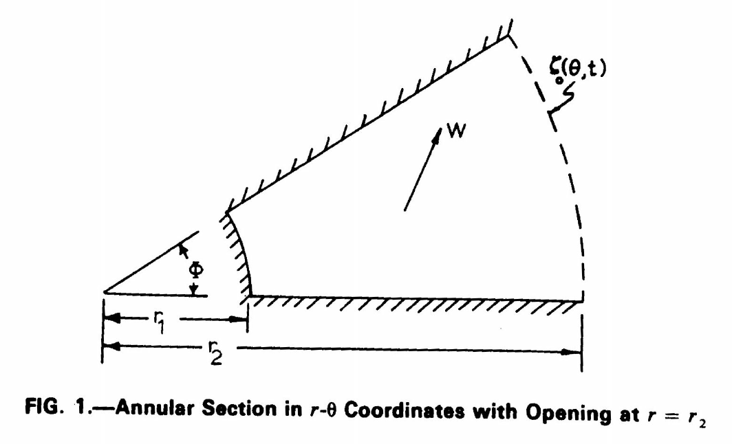
Wind Forcing on Polar Domain

We are interested in their solution for wind-driven flows on a polar domain, as shown below. Flow is required to be tangential to the solid boundaries at $r = r_1$ , $\theta = 0$ , and $\theta = \phi$ , where $\phi$ is arbitrary. For the wind-only case, the water levels are pinned at the outer boundary, $\zeta \left( r = r_2 \right) = 0$ . A constant wind stress $\mathbf{W}$ is applied in an arbitrary direction. Bathymetry is described by $h = H_0 r^{n}$ , in which $H_0$ is constant and $n$ may assume any real value.

Original Solution

A boundary-value problem is defined on this polar domain, and then a solution is derived by using separation of variables, an assumed form, and a Fourier series. The solution is drived fully for a wind stress acting in the $\theta = 0$ direction (i.e. toward the right in the figure), but then the solution is generalized for a wind stress with arbitrary direction:

$\begin{equation*} \mathbf{W} = W_0 \mathbf{r}_0 + W_\phi \mathbf{r}_\phi \end{equation*}$

in which $W_0$ and $W_\phi$ are the wind stress components in the $\theta = 0$ and $\theta = \phi$ directions. (For example, if $\phi = 90^\circ$ , then $W_\phi$ would act toward the top in the figure.) With this setup, they derive the analytic solution:

$\begin{equation*} \begin{aligned} \zeta_W \left( r , \theta \right) &= a^* r^{1-n} \left\{ W_0 \cos \left[ \kappa^* \theta \right] + W_\phi \cos \left[ \kappa^* \left( \theta - \phi \right) \right] \right\} \\ ~ &+ \sum_{j=0}^{\infty} \left\{ a_j r^{s_j} + b_j r^{t_j} \right\} \left\{ W_0 \cos \left( \frac{ j \pi \theta }{ \phi } \right) + W_\phi \cos \left[ \frac{ j \pi \left( \theta - \phi \right) }{ \phi } \right] \right\} \\ \end{aligned} \end{equation*}$

in which the coefficients $\left( a^* , \kappa^* , a_j , b_j , s_j , t_j \right)$ are defined in their paper (linked above). For example, the first coefficient is:

$\begin{equation*} a^* = \frac{ \sin \phi }{ g H_0 \kappa^* \sin \left( \kappa^* \theta \right) } \end{equation*}$

However, this solution is incorrect because it does not fully account for the arbitrary direction in these coefficients, which were derived only for the direction $\theta = 0$ . To account correctly for the additional component in the direction $\theta = \phi$ , the coefficients need to be re-defined, and the solution needs to be re-written.

Corrected Solution

That first coefficient should be:

$\begin{equation*} a_\alpha^* = \frac{ \sin \left( \theta - \alpha \right) }{ g H_0 \kappa^* \sin \left( \theta - \alpha \right) } \end{equation*}$

in which the numerator is now a function of direction $\theta$ , and $\alpha$ can be either $\alpha = 0$ (for $W_0$ ) or $\alpha = \phi$ (for $W_\phi$ ). This correction must be carried through the other coefficients $a_j$ and $b_j$ .

The correct analytical solution should be:

$\begin{equation*} \begin{aligned} \zeta_W \left( r , \theta \right) = r^{\left(1-n\right)} &\left\{ a_0^* W_0 \cos \left( \kappa^* \theta \right) + a_\phi^* W_\phi \cos \left( \kappa^* \left( \theta - \phi \right) \right) \right\} \\ ~ + \sum_{j=0}^{\infty} &\left\{ \left( a_{j,0} r^{s_j} + b_{j,0} r^{t_j} \right) W_0 \cos \left( \frac{ j \pi \theta }{ \phi } \right) \right. \\ &~ + \left. \left( a_{j,\phi} r^{s_j} + b_{j,\phi} r^{t_j} \right) W_\phi \cos \left( \frac{ j \pi \left( \theta - \phi \right) }{ \phi } \right) \right\} \end{aligned} \end{equation*}$

which accounts correctly for the contributions to the water levels from the two wind stress components. With this corrected solution, the water levels should respond correctly inside this polar domain.

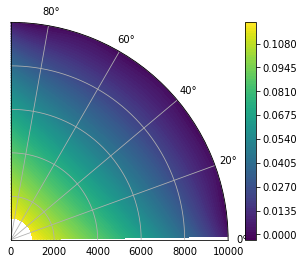
Example

We considered a simple test case with the following parameters:

$\begin{equation*} \begin{aligned} r_1 &= 1~\text{km} \\ r_2 &= 10~\text{km} \\ \phi &= 90^\circ \\ H_0 &= 100~\text{m} \\ n &= 0 \\ W_0 &= -0.01~\text{m}^2/\text{s}^2 \\ W_\phi &= -0.01~\text{m}^2/\text{s}^2 \\ \end{aligned} \end{equation*}$

so the domain is a quarter annular harbor with a constant bathymetry, and the wind stress is acting toward the bottom left. The water levels show a setup in the lower-left of the domain, with peaks of about 12 cm:

References

DR Lynch, WG Gray (1978). “Analytic Solutions for Computer Flow Model Testing.” Journal of the Hydraulics Division, ASCE, 104(10), 1409-1428.