
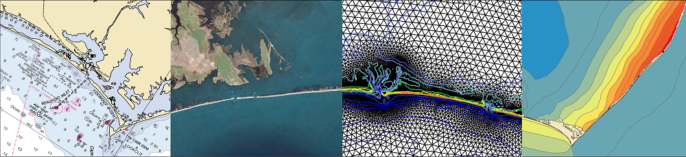
FigureGen is a FORTRAN program that creates images for ADCIRC files. It reads output files (fort.63, fort.64, maxele.63, etc.), grid files (fort.14, etc.), nodal attributes files (fort.13), etc. It plots contours, contour lines, and vectors. Using FigureGen, you can go directly from the ADCIRC input and output files to a presentation-quality figure, for one or multiple time snaps, without having to use SMS.
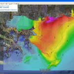
The following example depicts the water levels in ArcGIS as Ike moved through the Gulf:
Contours of water levels (m) in the Gulf of Mexico during Ike (2008), as visualized in ArcGIS.
This program started from a script written by Brian Blanton, and it contains code written by John Atkinson, Howard Lander, Chris Szpilka, Zach Cobell, and others. I converted it to FORTRAN because I am more familiar with that language, and I added the capability to plot vectors, among other things. But, at its core, FigureGen behaves like a script, and it uses system calls to tell other software how to generate the figure(s).
Note to Existing Users:
FigureGen v.41 requires you to upgrade your installation of GMT to version 4.5 or higher! We make use of their ps2raster command to convert the GMT PostScript files into raster images for use in presentations and publications, and this ps2raster command was not fully supported until GMT 4.5. So the bad news is that you will have to re-install that software in order to use this latest version of FigureGen. However, the good news is that we no longer need ImageMagick, so there is one less piece of software to worry about in the long run.
Also, FigureGen is backward-compatible! The input file changed slightly for this latest version, but you do not need to go back to your existing input files and update them. Instead, you can still use those input files with the new version to produce the same images as before. To do this, simply change the names of those existing input files so that the first four characters in the file name are FG and then the version number of FigureGen with which they correspond. For example, if you have an existing input file named Katrina_Ele-Wind.inp that worked with FigureGen v.26, then you can use that same input file with the new version by changing its name to FG26_Katrina_Ele-Wind.inp. That is the only change; you do not need to make any changes inside the input file itself. FigureGen v.41 will see that it is an older version of the input file, and it will not try to read the new lines for the new features.
Examples of New Features in v.41:
21. Read ADCIRC Output Files on the Fly. Now you can couple loosely FigureGen with an ADCIRC simulation and create images as the simulation is running. FigureGen will try to read data from your specified files (fort.63, fort.74, etc.), but it will not die if the data has not yet been written. Instead, it will output a message like:
Processor 0003 is trying to read from the end of fort.63.
Then it will wait a minute and try again. In this way, your ADCIRC simulation can be running and writing the files, FigureGen can be reading the files and generating images, and you will have a full set of images ready for you when your simulation is complete.
Note that, if you see that message and you’re not trying to run FigureGen concurrently with ADCIRC, then you know something is wrong with your FigureGen input file. Either you are trying to plot a time snap that doesn’t exist, or you’ve set something else incorrectly. Double-check that your existing ADCIRC files contain the time snaps that you’re trying to visualize.
 20. Geo-referenced JPG Images. We can generate JPG images with one or more layers, for one or more time snaps, and also generate the world files for geo-referencing. The image at right shows the wind reduction factors being used with ArcGIS. I have visualized the factors for all 12 directions, but we could do the same thing with multiple time snaps from an ADCIRC output file.
- FG41_20_Files
- FG41_20_WindRed_SL15v7l_SELA_GRF.inp
- Default2.pal
Note that the input file looks as it would if we were generating a regular figure. The only changes occur near the bottom of the input file, on the line where the GIS is activated. Note that setting the GIS flag to unity will produce one or more geo-referenced JPG images, while setting the GIS flag to two will also ZIP these images into one file. Also, note that we can specify the lowermost layer for each time snap, or we can allow FigureGen to select an optimal lowermost layer. (This behavior is slightly different than for the Google KMZ files in Example 18, in which we can specify the total number of layers. For the geo-referencing, only the topmost and lowermost layers will be generated.) Zach Cobell implemented this feature.
In this example, I have set the GIS flag to two, and I have specified that the lowermost layer be the second layer, both to speed up the run and to keep the ZIP file size manageable. So the resulting ZIP file contains geo-referenced JPG files for the top layer and the second layer. These files can then be pulled into ArcGIS or any similar program.
 19. Geo-referenced JPG Images. We can generate JPG images with one or more layers, for one or more time snaps, and also generate the world files for geo-referencing. The image at right shows geo-referenced JPG images of the maximum water levels during Katrina being used with ArcGIS.
- FG41_19_Files
- FG41_19_Katrina_MaxEle_SELA_GRF.inp
- Default2.pal
- 19_Katrina_MaxEle_SELA_GRF.zip
Note that the input file looks as it would if we were generating a regular figure. The only changes occur near the bottom of the input file, on the line where the GIS is activated. Note that setting the GIS flag to unity will produce one or more geo-referenced JPG images, while setting the GIS flag to two will also ZIP these images into one file. Also, note that we can specify the lowermost layer for each time snap, or we can allow FigureGen to select an optimal lowermost layer. (This behavior is slightly different than for the Google KMZ files in Example 18, in which we can specify the total number of layers. For the geo-referencing, only the topmost and lowermost layers will be generated.) Zach Cobell implemented this feature.
In this example, I have set the GIS flag to two, and I have allowed FigureGen to determine that the optimal lowermost layer is three. So the resulting ZIP file contains geo-referenced JPG files for the top layer and the third layer. These files can then be pulled into ArcGIS or any similar program.
 18. Creation of Google KMZ File with Multiple Layers. Create a Google KMZ file with one or multiple images, each with multiple layers. Note that the input file looks as it would if we were generating a regular figure. The only changes occur near the bottom of the input file, on the line where the Google flag is activated.
- FG41_18_Files
- FG41_18_Ike_EleDiff-Wind_GOMEX_KMZ.inp
- GMT_CorpDiff.cpt
- MaxEleDiff.txt
- CHL_New.png
- 18_Ike_EleDiff-Wind_GOMEX_KMZ.kmz
Note that we specify a transparency of 75 percent for the contoured image. Also, we add our lab logo by using the CHL_New.png file and activating the logo flag in the input file. And now we can also specify the number of layers per image. In this case, we are visualizing the wave setup during Hurricane Ike at 2008/09/12/1800Z, and we are applying five layers of images. Note how, in the animation at right, the resolution of the images does not deteriorate as we zoom into the map. Google Earth will select the layer of images that is appropriate for your zoom level.
Also note that the resolution of the image in the KMZ file is controlled by the “Resolution (dpi) of raster images.” line in the input file. For this layered image, I set the resolution as 100dpi, to control the overall KMZ file size.
I stole (shamefully) this KMZ technology from scripts that were written by Howard Lander at UNC. Those scripts are available on the ADCIRC Utility Programs page, and I highly recommend you check them out. In addition to the KMZ features shown here, those scripts can read and process binary output from ADCIRC.
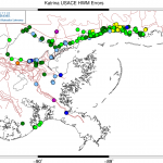 17. Errors from a HWM File in CSV Format. Plot the errors at a set of high-water marks (HWMs) based on information in a comma-separated value (CSV) file. The result is a graphical representation of where the errors are located and how bad they are. The example image shows the errors from our loosely-coupled hindcast of Katrina at the 206 HWMs collected by the US Army Corps of Engineers in Louisiana, Mississippi and Alabama.
- FG41_17_Files
- FG41_17_Katrina_USACE_SELA.inp
- HWM.cpt
- CHL_New.eps
These HWMs are specified as a CSV file with the following format:
lon,lat,bath,measured,modeled,error
but it only reads the first, second and sixth columns. We also make the following changes to the FigureGen input file: turn off the filled contours and contour lines, set the contour file format to HWM-CSV, specify a special HWM.cpt color palette, and set the number of times to split intervals at unity. (This last setting will remove the smoothness in the color palette and establish clear bins for the different errors.)
 16. Color Palettes in CPT Format. In addition to the support for the PAL format used by SMS, FigureGen now supports color palettes in the CPT format. This palette format can be used in the same way as before: either by itself, or in combination with a text file to specify the exact intervals in the scale. GMT uses the CPT format internally, so I was always converting the PAL format before using it with GMT to make the images. Now you can skip that step if you have a pre-existing CPT file.
- FG41_16_Files
- FG41_16_Katrina_MaxEleDiff_SELA.inp
- GMT_CorpDiff.cpt
- CHL_New.eps
 15. High-Resolution Coastlines and Inland Water Bodies. Use the built-in GMT
 pscoast command to add high-resolution coastlines and water-body outlines to plots. Note that the coastline and inland water bodies are controlled on a line near the bottom of the input file. If the flag is set to 1, then these outlines will be added to the figure in the user-specified color. You can specify one of four levels of resolution for these outlines; at the highest resolution (4), the coastlines are added with intricate detail. The example GIF shows how the resolution can vary. Over a small geographic region, it is best to use the highest resolution. However, over large regions, it might be faster to use a lower resolution without any noticeable effect on quality. Zach Cobell implemented this feature.
- FG41_15_Files
- FG41_15_ManningsN_SL15v7l_SELA.inp
- Default2.pal
- CHL_New.eps
Examples of Previous Features:
 14. Creation of Google KMZ File for a Time Series of Images. Create a time series of images (of the water levels and winds during Hurricane Katrina, in this case), and then write a KMZ file that can be used in Google Earth. Note that the input file looks as it would if we were generating a regular figure.
- FG41_14_Files
- FG41_14_Katrina_Ele-Wind_SELA_KMZ.inp
- Default2.pal
- CHL_New.png
- 14_Katrina_Ele-Wind_SELA.kmz
The only changes occur near the bottom of the input file, on the line where the Google flag is activated. Note that we specify a transparency of 75 percent for the contoured image. Also, we add our lab logo by using the CHL_New.png file and activating the logo flag in the input file. FigureGen will automatically strip away the boundary of the image, and it will create the contour scale and the logo as separate layers in the KMZ file.
Also note that we specify a time stamp (in the format YYYYMMDDHHMMSS) that corresponds to the time of the first snap in the fort.63 file. FigureGen will use that time stamp and the information in the fort.63 file to determine the times of all of the rest of the snaps. Then it will add a realistic time bar to the top of the KMZ file.
Also note that the resolution of the image in the KMZ file is controlled by the “Resolution (dpi) of raster images.” line in the input file. For this animation, I changed the resolution to 100dpi, so that the corresponding KMZ file does not become too large. For KMZ files containing a single image (as in Example 13, below), the resolution can be increased to control the overall KMZ file size.
I stole (shamefully) this KMZ technology from scripts that were written by Howard Lander at UNC. Those scripts are available on the ADCIRC Utility Programs page, and I highly recommend you check them out. In addition to the KMZ features shown here, those scripts can read and process binary output from ADCIRC.
 13. Creation of Google KMZ File for a Single Image. Create a single image (of the maximum water levels during Hurricane Katrina, in this case), and then write a KMZ file that can be used in Google Earth. Click on the image at right to download the KMZ file and use it with Google Earth on your computer. Note that the input file looks as it would if we were generating a regular figure.
- FG41_13_Files
- FG41_13_Katrina_MaxEle_SELA_KMZ.inp
- Default2.pal
- CHL_New.png
- 13_Katrina_MaxEle_SELA.kmz
The only changes occur near the bottom of the input file, on the line where the Google flag is activated. Note that we specify a transparency of 75 percent for the contoured image. Also, we add our lab logo by using the CHL_New.png file and activating the logo flag in the input file. FigureGen will automatically strip away the boundary of the image, and it will create the contour scale and the logo as separate layers in the KMZ file.
Also note that the resolution of the image in the KMZ file is controlled by the “Resolution (dpi) of raster images.” line in the input file. For this single image, I set the resolution as 200dpi, because that is the highest resolution where GMT will still be able to make transparent the white space at the border of the image. For KMZ files containing animations (as in Example 14, above), the resolution should also be decreased to control the overall KMZ file size.
I stole (shamefully) this KMZ technology from scripts that were written by Howard Lander at UNC. Those scripts are available on the ADCIRC Utility Programs page, and I highly recommend you check them out. In addition to the KMZ features shown here, those scripts can read and process binary output from ADCIRC.
 12. Domain Decomposition. Read the
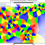
 partmesh.txt file that is output from ADCPREP and plot the domain decomposition. Note that we specify the partmesh.txt file as the contour file, and we set the contour file type to GRID-DECOMP-256, where the last number is the total number of processors. FigureGen will read the grid file and partmesh.txt file, and then it will apply an optimal color connectivity table so that no two adjoining subdomains will receive the same color. In this example, the number of colors is six. I think the theoretical minimum number of colors is four for such a mapping exercise, but that algorithm is too costly for FigureGen.
- FG41_12_Files
- FG41_12_Grid-Decomp_SL15v7l_SELA.inp
- Decomp.pal
- CHL_New.eps
Also note that, in this example, we are coloring the mesh lines in each subdomain (as in Examples 7 and 6, below). This is accomplished by: (A) turning on the plot grid flag, (B) turning off the contour fill flag, and (C) setting the color lines flag to GRID-DECOMP-256. A different combination of settings could produce a similar image, except the subdomains would be colored as filled contours.
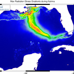 11. Add connected Hurricane Track, Logo to plot of Maximum Wave-Driven Forces. Above a plot of the contours from the
 maxrs.63 output file, add the connected track of Hurricane Katrina and a logo. Note that this example contains two features. First, we are plotting the track of Hurricane Katrina (from KatrinaTrack.txt) as a set of connected line segments. This was not possible in v.26, which required that the dots in such a file be unconnected, and thus made it difficult to add lines such as hurricane tracks to the figures. Now, by setting the dots/lines flag to 2 near the bottom of the input file, you can connect the dots.
- FG41_11_Files
- FG41_11_Katrina_MaxRS_GOMEX.inp
- Default2.pal
- RS_Intervals.txt
- KatrinaTrack.txt
- CHL_New.eps
Second, note that we are adding our lab logo to the top left corner of the figure. This is done on a new line in the input file for v.32. You can specify the location of the logo (TL/TR/BL/BR), the width of the logo in inches, and the name of the EPS logo image that you want to add. Please note that GMT requires the logo to be in EPS format. This was not my choice. However, I think that most high-end image software should allow you to save or convert an image to EPS format.
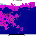 10. Eddy Viscosity from the
 fort.13 File. Read the ADCIRC nodal attributes file and plot the eddy viscosity values. Note that we specify the fort.13 file as the contour file, and we set the format to “13-EVIS.” We can plot the wind reduction factors, canopy values, eddy viscosity, and tau0 using similar commands.
- FG41_10_Files
- FG41_10_EVis_SL15v7l_SELA.inp
- Default2.pal
- CHL_New.eps
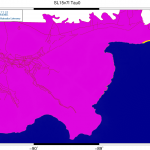 9. Tau0 from the
 fort.13 File. Read the ADCIRC nodal attributes file and plot the tau0 values. Note that we specify the fort.13 file as the contour file, and we set the format to “13-TAU0.” We can plot the wind reduction factors, canopy values, eddy viscosity, and tau0 using similar commands.
- FG41_09_Files
- FG41_09_Tau0_SL15v7l_SELA.inp
- Default2.pal
- CHL_New.eps
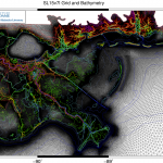 8. Grid and Colored Contour Lines of Bathy/Topo. Read an ADCIRC grid file and plot the grid itself. Add contours, and color them based on the bathymetry/topography itself. Note that this plot combines two new features. First, the grid is plotted by turning on the plot grid flag in the input file. The grid can be combined with the other options in FigureGen, including contours, contour lines, etc.
- FG41_08_Files
- FG41_08_Grid-Contours_SL15v7l_SELA.inp
- TopoRainbow.pal
- TopoRainbow.txt
- CHL_New.eps
Second, the bathymetry/topography contour lines are plotted by specifying the grid file as the contour file, setting the contour file format to GRID-BATH, and setting the color lines flag to CONTOUR-LINES. This combination of settings tells FigureGen to read the grid file and plot the contour lines of bathymetry/topography. The last setting tells FigureGen to use the color palette on the contour lines, instead of plotting them in black. Note that the color lines flag requires GMT 4.3.0.
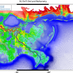 7. Grid with Bathy/Topo Coloring. Read an ADCIRC grid file and plot the grid itself. Instead of black lines, color the grid lines based on the bathymetry/topography. Note that we must combine several settings to produce this plot. The plot grid flag is activated, all of the contours are deactivated, the grid file is specified as the contour file, and the contour file format is set to
 GRID-BATH. Finally, we also set the color lines flag to GRID-BATH. This setting tells FigureGen to color the grid lines based on the bathymetry. (Alternatively, we could generate a similar plot of the grid sizes by changing these settings to GRID-SIZE.) Note that the color lines flag regures GMT 4.3.0.
- FG41_07_Files
- FG41_07_Grid-Bath_SL15v7l_SELA.inp
- TopoRainbow.pal
- TopoRainbow.txt
- CHL_New.eps
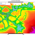 6. Contours of Grid Sizes. Read an ADCIRC grid file and plot contours of the grid sizes. Note that the grid file is also specified as the contour file, and then the contour file format is set to
 GRID-SIZE. This tells FigureGen to compute the grid sizes as it reads the grid file. GMT needs contour data at the nodes, so the grid sizes are averaged onto each node before plotting.
- FG41_06_Files
- FG41_06_Grid-Size_SL15v7l_SELA.inp
- Default2.pal
- GridSize.txt
- CHL_New.eps
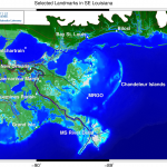 5. Bathy/Topo Contours with Labels of Landmarks. Read an ADCIRC grid file and plot contours of the bathymetry/topography. Then add labels as directed by an external file. Note that the labels are controlled by a line near the bottom of the input file. The user can specify the color and the file name of the labels. This external file contains the longitudes, latitudes, text sizes, rotation angles, font numbers (from GMT), justifications, and text. Note that the justification is a two-letter combination of Left/Center/Right and Top/Middle/Bottom.
- FG41_05_Files
- FG41_05_Bath_SL15v7l_SELA.inp
- TopoBlueGreen.pal
- TopoBlueGreen.txt
- Labels.txt
- CHL_New.eps
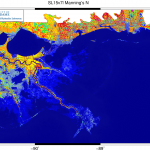 4. Manning’s n from the
 fort.13 File. Read the ADCIRC nodal attributes file and plot the Manning’s n values. Note that we specify the fort.13 file as the contour file, and we set the format to 13-MANNING. We can plot the wind reduction factors, canopy values, eddy viscosity, and tau0 using similar commands.
- FG41_04_Files
- FG41_04_ManningsN_SL15v7l_SELA.inp
- Default2.pal
- CHL_New.eps
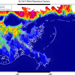 3. Wind Reduction Factors from the
 fort.13 File. Read the ADCIRC nodal attributes file and plot one or more columns of the wind reduction factors. Note that we specify the fort.13 file as the contour file, and we set the format to 13-WIND-REDUCTION-4. The last number in that string specifies the column to plot, so we are plotting the wind reduction factors from the fourth column (which corresponds to northward winds).
- FG41_03_Files
- FG41_03_WindReduction_SL15v7l_SELA.inp
- Default2.pal
- CHL_New.eps
To plot all 12 columns, set the contour file format to 13-WIND-REDUCTION. Then, if you have installed ImageMagick, then you can use the following command:
convert *.jpg WindReduction.gif
to create an animation. Also note that we are adding a white coastline to the figure. However, we are doing it in a different manner than in previous versions of FigureGen, which used the dots/lines flag to specify an external file with lat/lon coordinates of the coastline. Now, we can use the built-in GMT coastline feature; see the example above.
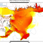
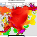 2. Difference Plots. Read ADCIRC files and plot contours of the differences between the two files. If the files have the same number of nodes, then this feature will work on output files, grid files (for bathymetry only), and
 fort.13 files. In this example, we plot the differences between the maximum water levels from a fully coupled simulation and a simulation without wave effects. This is comparable to a wave set-up, although it is important to remember that the tides can muddy the picture when we look at the maximum water levels. It is best to compute wave set-up on a snap-by-snap basis.
- FG41_02_Files
- FG41_02_Katrina_MaxEleDiff_SELA.inp
- Default2.pal
- MaxEleDiff.txt
- CHL_New.eps
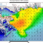 1. Hurricane Water Levels and Winds. Read ADCIRC output files and plot the contours of water levels and vectors of winds. Note that FigureGen accepts a broad range of ADCIRC output files. Anything that is formatted like a
 fort.63 or fort.64 file will work for the contours, and anything that is formatted like a fort.64 file will work for the vectors.
- FG41_01_Files
- FG41_01_Katrina_Ele-Wind_SELA.inp
- Default2.pal
- CHL_New.eps
System Requirements:
1. GMT
GMT is the software package that plots the contours, contour lines, etc and produces a PostScript file (*.ps) containing the figure. The GMT software package is actually a suite of executable programs, of which FigureGen uses only a subset. Note that FigureGen v.41 only works with GMT 4.5 or higher! We now use their ps2raster command to convert the PostScript files to raster images, and the ps2raster command was not fully implemented until GMT 4.5. However, because of this, we now do not need ImageMagick at all.
2. GhostScript
GhostScript is the software package that converts PostScript files into different formats, including the raster format used by FigureGen. GhostScript is typically installed on Unix systems, so it may already be available on your system.
Source Files:
The FigureGen program requires a source file and accompanying input files. These files are linked here:
This is the source code itself. This code will ask the user for and then read an input file containing information about which files to plot and how. FigureGen will plot the contours of both elevation-type (fort.63, maxele.63, maxwvel.63, etc.) and velocity-type (fort.64, fort.74, etc.) output files, grid (fort.14) files, and nodal attributes (fort.13) files. You can specify a color palette to use by creating and saving a palette in SMS. You can convert units automatically. You can specify the lat/lon box to plot. And, perhaps most importantly, you can run FigureGen in parallel, so that you can create multiple images in a short amount of time. This source code contains directives for both serial and parallel compilation, and directions on how to compile are included below.
2. Input File
The input file contains all of the buttons and levers that you can adjust for your figures. You can change the lat/lon boundaries of the box; you can turn on/off the contours, contour lines, vectors, etc.; you can convert the units in the ADCIRC output files; you can create figures for several time snaps; you can control the appearance of the scale; etc. Example input files are linked above.
3. Default2.pal
You can control the colors in FigureGen by specifying the name of a color palette in the input file. This color palette was created and saved from SMS, and it is the palette that we use for our hindcast figures. If you wanted a different palette, then you can use SMS to create one, and then use FigureGen to apply it to figures.
4. Contour Increments File
You can control the increments in the contour scale by specifying a text file with the increments you want. The first line in the file contains the number of increments in the file. The rest of the lines in the file have two numbers: (A) the increments that you want to use, and a flag (0 or 1) to indicate whether the color in that increment should be superseded by gray. (For example, you might want to make the increment near zero to be gray, especially in a difference plot.) Examples of this file are linked above.
How to Compile:
As stated above, FigureGen is written so that the source file contains instructions for both serial and parallel implementations. For that reason, it may not be straight-forward to compile. Here is what has worked for me:
1. Serial compilation using the Absoft FORTRAN compiler (on Athos):
f90 FigureGen41.F90 /Applications/Absoft/lib/libU77.a -o FigureGen41.exe
Now the compiler knows automatically to use the pre-processor, but we have to specify two other things. First, we need to include the library of Unix commands. The FigureGen program relies heavily on calls to the operating system, and these calls are not defined automatically by the Absoft FORTRAN compiler. Second, we need to specify the name of the executable by using the -o option.
2. Parallel compilation using the Absoft FORTRAN compiler and LAM/MPI (on Athos):
mpif77 FigureGen41.F90 -DCMPI -I$LAMHOME/include -o FigureGen41.exe
The -DCMPI flag turns on the parallel commands inside my FORTRAN source file. The -I option specifies the location of the LAM/MPI include directory, where my code uses the mpif.h library. And the -o option specifies the name of the executable to be created.
3. Serial compilation using the Portland Group compilers (on Zas):
pgf90 FigureGen41.F90 -o FigureGen41.exe
The only trick here is that we need to specify the name of the executable to be created by the compilation.
4. Parallel compilation using the Portland Group compilers and MVAPICH (on Zas):
mpif90 FigureGen41.F90 -DCMPI -o FigureGen41.exe
The -DCMPI flag turns on the parallel commands inside my FORTRAN source file. And the “-o” option specifies the name of the executable to be created.
That is all of the experience that I have in compiling FigureGen. It seems that the main difficulties are: (A) ensuring that the compiler uses its pre-processor to handle the compiler directives, (B) linking to the Unix library that contains the definitions for the system calls, (C) defining the flag to turn on the parallel commands in my source code, and/or (D) specifying the directory where the MPI library is located. If your experience is different, then please let me know.
How to Run:
In a serial implementation, running FigureGen is easy. Typing the name of the executable will start the program. It will ask the user for the name of the input file, which it will then read and process. From that point forward, the rest of the figure generation is automatic.
In a parallel implementation, I use the following steps. On our system, the command to run a parallel program on three processors is:
mpirun -ssi rpi tcp c0,1-2 -x PATH ./FigureGen41.exe
Note that I am being very specific about which processors I request. The first processor in the list will be the master in my master-slave paradigm. And, because FigureGen is interactive (by asking for the name of the input file), I always ask for processor 0 to be the master because that is the processor from which I perform the run. The rest of the processors will be the slaves, and they will make the figures. In the line above, I am requesting that processors 1 and 2 be the slaves. If I wanted to split the work amongst 10 processors, I might use a command like:
mpirun -ssi rpi tcp c0,21-30 -x PATH ./FigureGen41.exe
where now I am requesting that processors 21 through 30 be the slaves. The master will assign a time snap to each slave and then wait to hear back from the slaves. When a slave is finished generating a figure for the time snap it was assigned, then it will alert the master and receive a new time snap.
Also note that I am using the -x PATH option. This option exports the PATH environment variable to the compute nodes. I found it necessary to use this option because, even though I had set the paths to the ImageMagick and GhostScript executables, the compute nodes sometimes could not find them. By exporting these paths, we tell the compute nodes where the executables are located.
Troubleshooting:
Before running FigureGen, it is important that the necessary files be located in the working directory. Specifically, the grid file, the file from which to plot contours (if used), the file from which to plot vectors (if used), and the color palette (if used) should be in the same folder as the FigureGen executable. In addition, you will need to create the temporary folder that is named in the input file. This is where FigureGen will create any temporary files as it works. You can run multiple instances of FigureGen from the same folder by specifying separate temporary folders for each instance. Thus, you might be generating Ele-Wind figures using a temporary folder called Temp1 at the same time that you are generating Wind-Wind figures using a temporary folder called Temp2.
Also, on some systems, you cannot read in the same file for both contours and vectors. For example, to plot the hurricane winds, you might want to plot contours of wind magnitude and vectors of wind magnitude and direction. All of this information would need to come from the same fort.74 file, but you cannot specify the same fort.74 file for both the contours and vectors. The work-around is to copy the fort.74 file into a new fort.2.74 file, and then use one file for contours and the other file for vectors.