
We first noticed the problem while validating the computed SWAN significant wave heights against the measured results at eight gauges deployed by Notre Dame assistant professor Andrew Kennedy. These gauges were deployed in the days before Ike’s landfall along the Texas coastline, as shown below:
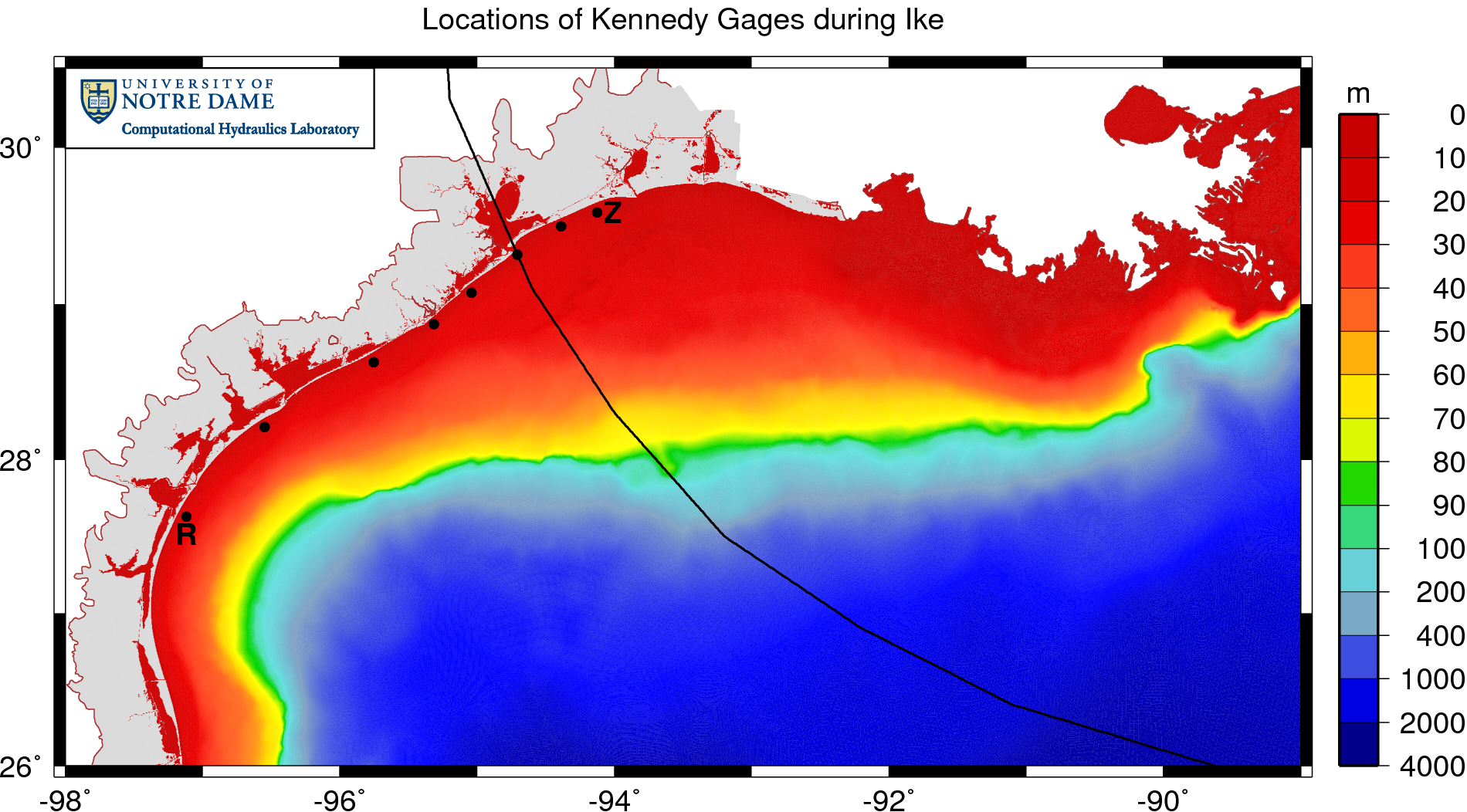
Locations of Kennedy gauges during Ike (2008).
Ike’s track is shown with a black line; note how the storm curved northwestward in the Gulf of Mexico and made landfall near Galveston and Houston. The eight gauges are shown with black dots, and are located very near the coastline in 10-20m of water depth. The information measured by these gauges is extremely valuable, especially with respect to wave validation, because the gauges are located nearshore, where the waves would feel the effects of bottom friction and depth-induced breaking.
Let’s focus our attention on the first and last gauges, labeled R and Z on the figure above. Gauge R was located far to the west of the track, near Corpus Christi. The winds were blowing offshore and relatively weak at this location, so the majority of the measured wave action was due to swell that propagated from the deeper water in the Gulf. In contrast, gauge Z was located east of the track, where it would have experienced the full strength of the hurricane winds. These winds would have blown onshore as the storm was making landfall, thus creating local wind-sea waves in addition to swell.
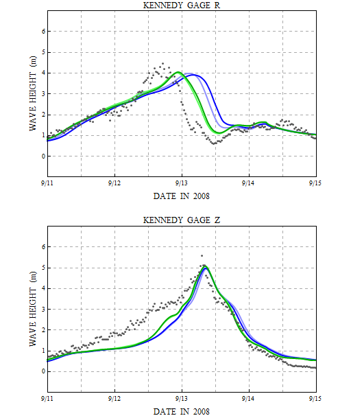
Our initial validation results are shown in the following figure. The measured significant wave heights are shown in black dots, while the computed SWAN results are shown in solid lines. The lighter blue line shows the results from a run on 1015 computational cores, while the darker blue line shows the results from the same run on 2039 cores.
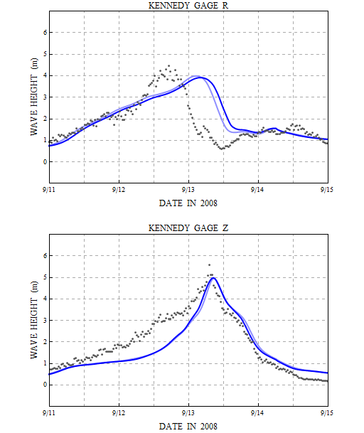
Significant wave heights (m) at two Kennedy gauges during Ike (2008) for simulations on 1015 cores (light blue) and 2039 cores (dark blue).
At gauge R, the response is due entirely to swell propagating from offshore, as the measured peak occurs 12-15 hours before landfall. The magnitudes of the computed SWAN significant wave heights are close to the measured values, but there is a significant phase lag. The peak in the SWAN solution occurs about 12 hours later than the peak in the measured values. And the lag is exacerbated when the mesh is decomposed over more computational cores; note how the darker blue line is shifted even farther to the right on the plot.
At gauge Z, the local wind-sea waves are modeled well by SWAN, both in magnitude and timing, and the solution does not depend on the domain decomposition. However, SWAN still misses the arrival of the swell waves before the storm. For most of the day on 12 August 2008, the modeled SWAN wave heights are 1-1.5m below the measured values.
This behavior suggests that the swell is not propagating correctly during this simulation. Our comparisons at the deep-water NDBC buoys showed good agreement, so we know that we are generating the swell in the Gulf. But something is slowing it down as it moves onto the continental shelf and into the nearshore. We varied the bottom friction formulation in our SWAN simulation, and that helped, but it did not solve the problem.
Then we noticed that the problem correlated strongly with the mesh resolution. On coarser meshes, such as our EC2001 mesh with its ~250K vertices, the swell propagated faster and the comparison to the measured data was good. The comparison was also better on earlier versions of the Texas mesh, which was also coarser. In later versions, though, we increased the resolution in the Gulf of Mexico, as shown in the figure below:
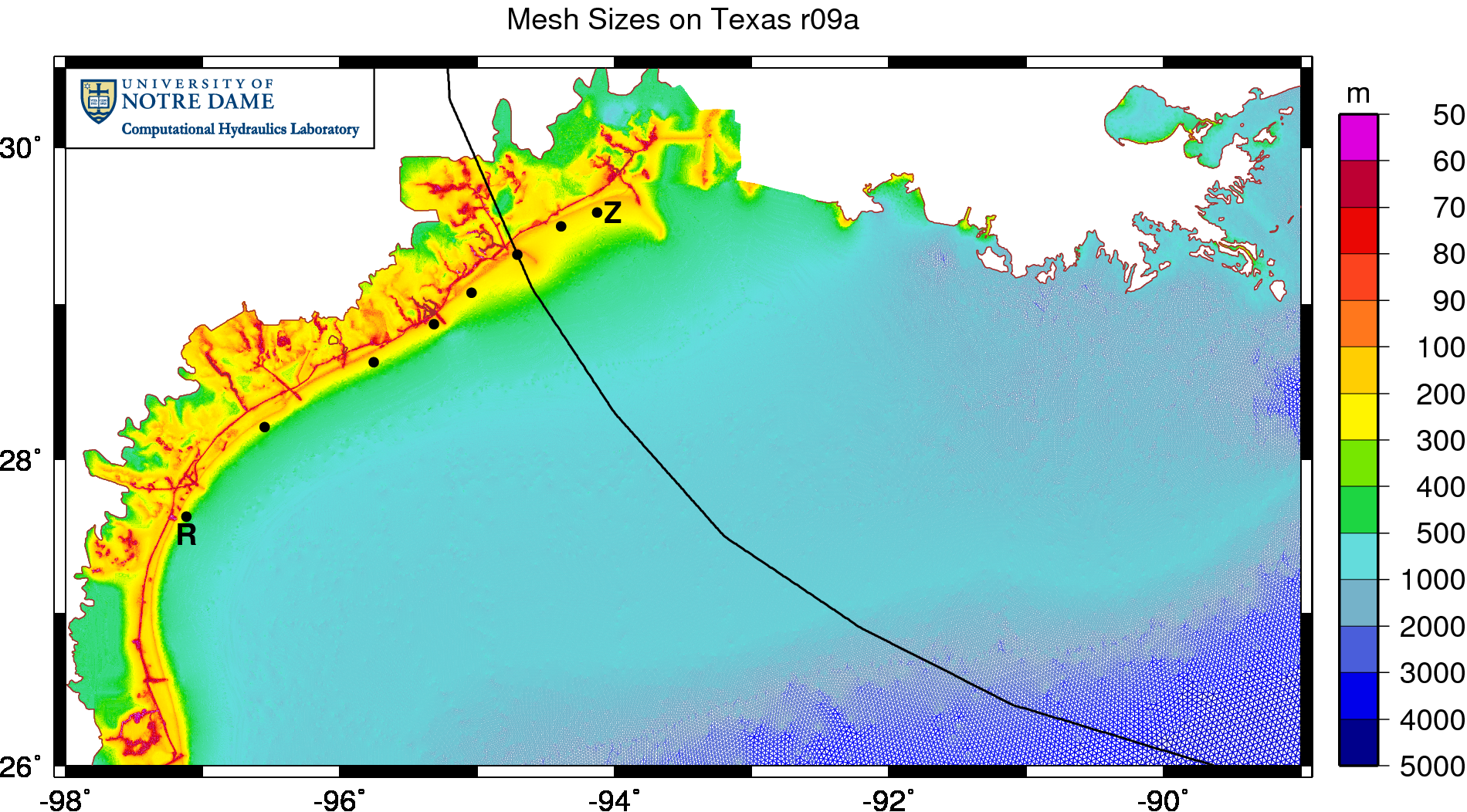
Element sizes (m) on the TX2008r09a mesh.
This version of the Texas mesh has ~3.3M vertices, many of which are employed in the Gulf to improve the wave solution. In previous meshes, the resolution was 12-18km in the middle of the Gulf, but we have reduced it to 4-6km to better model the generation of wave energy as the storm moves over deep water. On the continental shelf, the resolution decreases to about 500m-1km, and it is reduced further to 200m in the wave breaking zones. In fine-scale channels such as the GIWW and the Galveston Shipping Channel, the resolution varies down to 30m. This resolution allows SWAN+ADCIRC to capture features of both waves and surge.
However, the wave model only works as well as the wave modeler allows. We were using modified convergence criteria in SWAN that were not allowing the swell to propagate correctly on this fine mesh. Specifically, we were forcing SWAN to perform exactly two iterations per time step:
NUM STOPC DABS=0.005 DREL=0.01 CURVAT=0.005 NPNTS=101 NONSTAT MXITNS=2
The criteria related to the SWAN solution (DABS, DREL and CURVAT) are the default values suggested by the SWAN User Manual. But we adjusted the other criteria to require SWAN to iterate until the solution converged in 101 percent of the mesh vertices or it reached two iterations in a time step. Effectively, these criteria required SWAN to iterate exactly twice per time step. (The default values for the unstructured version of SWAN are NPNTS=99.5 and MXITNS=50.)
It is important to note that we did not pick these convergence criteria out of the air. During our validation hindcasts of Katrina and Rita on the SL15 mesh, we performed extensive tests on the convergence criteria and the coupling interval, and we found these values to be sufficient, i.e., the solution did not change when we tightened them. In addition, these convergence criteria had the benefit of balancing the time spent in SWAN and ADCIRC. One, 600-second SWAN time step with two iterations was about as costly as 600, one-second ADCIRC time steps. The total run-time roughly doubled.
Detailed, nearshore measurements of swell were not available for Katrina and Rita, so it was impossible to validate in that respect. But the resolution in our earlier meshes would have allowed for better swell propagation. The SL15 mesh has a coarser representation of the deeper Gulf and the continental shelf, with the mesh sizes ranging to 12-18km in the middle of the Gulf. It was only when we refined the mesh in those regions that we started to slow the swell.
In the early stages of the hindcast simulation, when the hurricane is far away and the wave solution is not changing rapidly, the convergence criteria may be over-restrictive. SWAN may only need to iterate once per time step during that stage of the simulation. However, as the storm moves toward its landfall, it would require more iterations per time step, especially to propage the relatively fast-moving swell. This problem is exacerbated on fine meshes, because of the structure of the SWAN code:
DO IT=1,NumTimeSteps

    DO IR=1,MXITNS

       DO IS=1,NumSweeps

          Gauss-Seidel Sweeping of Wave Action Density

          If Updated, Then Exit IS Loop

       ENDDO

       Exchange Information At Sub-Mesh Boundaries

       If Converged, Then Exit IR Loop

    ENDDO

ENDDO
To greatly over-simplify things, the SWAN code is structured like a nested DO loop with three levels. Each time step has a loop over one or more iterations, and each iteration has a loop over at least two sweeps. When the wave energy has been updated within each sub-mesh, then the code exits the sweeping loop. And, when the wave energy has converged on the global mesh, then the code exits the iterating loop.
Note that information is passed between neighboring sub-meshes at the end of each iteration. By limiting our simulation to two iterations, we were limiting the passing of information and thus the propagation of wave energy between local sub-meshes. The swell was slowed numerically as it moved from the deep water onto the continental shelf. This problem was most evident on our latest version of the Texas mesh, when we increased the resolution offshore, and thus decreased the geographical area of each local sub-mesh:
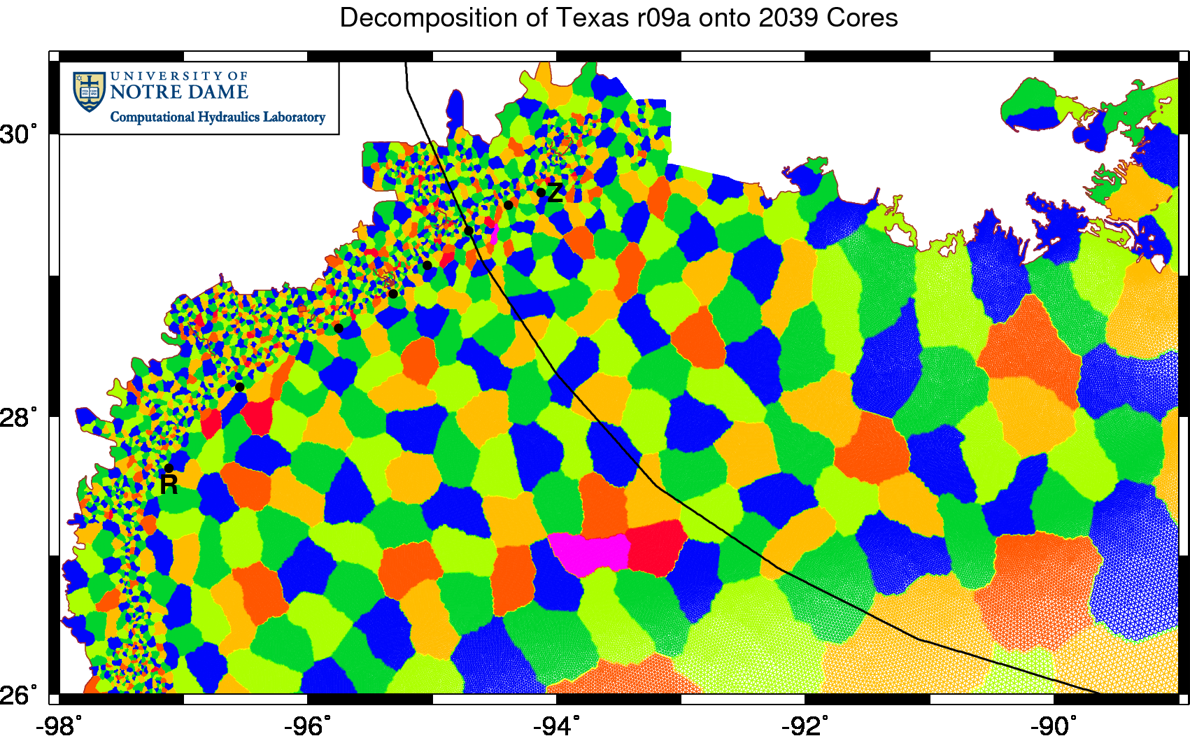
Example decomposition of the TX2008r09a mesh onto 2039 cores.
This figure shows the decomposition of the Texas r09a mesh onto 2039 computational cores. Each core runs SWAN+ADCIRC on a local sub-mesh, shown in varying colors in the figure. The goal is to keep constant the number of mesh vertices on each sub-mesh, so the sub-meshes decrease in geographical size as the average mesh size decreases. That is why the sub-meshes are so small overland in Texas. But they are also relatively small offshore. Similar plots of earlier meshes, such as EC2001, SL15 or earlier versions of the Texas mesh, would show much larger sub-meshes on the continental shelf.
Information is passed across the boundaries of the sub-meshes. However, when we limited SWAN to two iterations per time step, we also limited this passing of information. The increased resolution on the continental shelf caused the sub-meshes to be smaller, thus slowing the propagation of the swell. We fixed this problem by using convergence criteria that are closer to the recommendations on the SWAN User Manual:
NUM STOPC DABS=0.005 DREL=0.01 CURVAT=0.005 NPNTS=95 NONSTAT MXITNS=20
So now we require the solution to converge in 95 percent of the mesh vertices or within 20 iterations per time step, whichever comes first. When the solution is changing rapidly, such as after a cold start or during the peak of the storm, then the solution may require all 20 iterations. But during the rest of the simulation, SWAN will meet the convergence criteria in fewer iterations.
Note that we are not changing the physics of the simulation, only its numerics. These new convergence criteria allow the wave energy to propagate better through the domain, because we are passing information between sub-meshes as much as necessary. The improvement is evident when we compare to Dr. Kennedy’s gauge data, as shown in the figure below. Again, the measured significant wave heights are shown in black dots, while the computed SWAN results are shown in solid lines. The lighter green line shows the results from a run on 1015 computational cores, while the darker green line shows the results from the same run on 2039 cores.
Significant wave heights (m) at two Kennedy gauges during Ike (2008) for simulations with a maximum of 20 iterations.
At gauge R, note the significant improvement in the phasing of the swell at this location. Instead of lagging by 12 hours, the swell now lags by 4-6 hours. This result is still sub-optimal, so we continue to search for ways to improve it. However, further tightening of the convergence criteria, either by increasing the required percentage of converged mesh vertices or by increasing the maximum number of iterations per time step, does not improve the solution.
At gauge Z, the new convergence criteria do not change the solution significantly, although there is a noticeable bump in the swell about 12 hours before landfall. This is further evidence that the numerics are no longer slowing the propagation of the swell. However, at this location, the majority of the wave action is generated locally, and SWAN continues to show a good match to the peak of the significant wave heights.
These new convergence criteria had an effect on the run-times, increasing them by about 30 percent. That means the SWAN half of the coupled SWAN+ADCIRC model was 60 percent more costly. This price is worthwhile for the gain in accuracy.
Again, we recognize that these results are sub-optimal, in that they do not match perfectly the measured data at these locations. But now the numerics are no longer holding us back. We can focus on the physics of swell propagation. Maybe our bottom friction is too dissipative? Maybe our bathymetries are incorrect? There are many things we can learn as we become better wave modelers.