Integral Coupling of Bottom Friction | Coastal & Computational Hydraulics Team

Updated 2010/06/16: Revised figures from our Gustav MWR paper.
Updated 2011/08/26: Removed the Google Maps inset.
Updated 2012/09/10: Added the Google Maps inset and updated the equations in LaTeX.

One strength of the integral coupling of SWAN+ADCIRC is the increased accuracy resulting from the communication of the model components during the simulation. The computed wave solution is better because it includes the water levels and currents passed from ADCIRC, and the computed circulation solution is better because it includes the wave radiation stress gradients passed from SWAN. These benefits are described in a manuscript we submitted recently to Coastal Engineering (Dietrich et al., 2011).

We have applied SWAN+ADCIRC to the most recent hurricanes to impact southern Louisiana, including Gustav and Ike (2008). The following example shows the significant heights of the waves generated by Gustav as it moved through the Gulf:

gustav-hs-gomex

Note how the waves are generated in the deeper Gulf and then propagated onto the continental shelf, where they break due to changes in bathymetry and bottom roughness. The associated radiation stress gradients are passed from SWAN to ADCIRC and used to drive currents and set-up. Our new SL16 mesh contains significantly more resolution in all of the wave transformation zones, including mesh spacings of about 4km in deep water, 500m-1km on the entire shelf, and 100-200m in the breaking zones.

However, the water levels, currents and radiation stress gradients are not the only parameters that can be coupled integrally. This page describes how we have also coupled the bottom friction between the two model components. In SWAN, using the friction formulation of Madsen et al. (1988), we can vary the bottom rougness both spatially and temporally, by computing physical roughness lengths based on the Manning’s $n$ coefficients used by ADCIRC.

Motivation

In computing its friction coefficient, ADCIRC makes use of Manning’s $n$ values that are derived from land-cover databases. These data sets contain information about the land types throughout our study region, usually at a resolution that is finer than what we employ in SWAN+ADCIRC. We associate these land types with representative Manning’s $n$ values, and then we area-average them to our mesh vertices. John Atkinson did a lot of the early work to automate this process in southern Louisiana, and other people have expanded his work for different applications.

The example below shows the Manning’s $n$ values on our SL16 mesh, which has about 5M mesh vertices and resolves the geographical features in southern Louisiana down to about 30m.

manningsn-sl16-sela

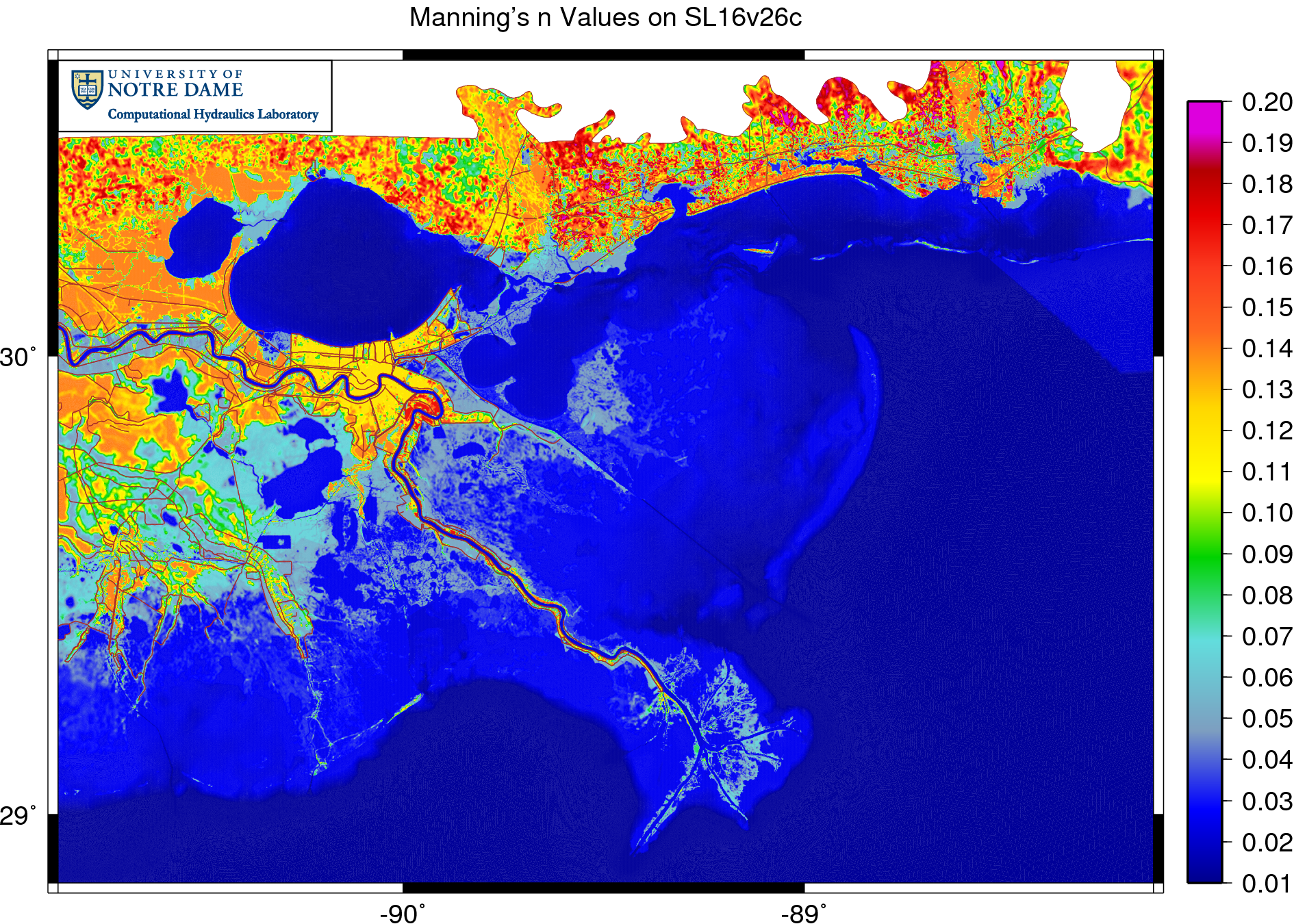
Note the spatial variability in this field. The Manning’s $n$ values are relatively small in the Gulf and on the continental shelf, but they increase in the marshes and floodplains of southern Louisiana. They are large in the residential areas near New Orleans and in the wooded regions of Mississippi and Alabama. In ADCIRC, as storm surge moves through this domain, it sees a different bottom friction depending on the local terrain.

However, in SWAN, we had been using the default JONSWAP formulation of friction, which does not vary spatially. We already have terrain-specific information in ADCIRC about the bottom friction, so it would be great if that information could also be utilized by SWAN to increase the accuracy of its wave computations. The result would be a friction formulation that is tied to the local bathymetry and topography.

Formulation

As noted in the SWAN User Manual, bottom friction is formulated as a dissipation term and included as part of the source/sink term in the spectral action balance equation. It has the form:

$\begin{equation*} S_{ds,b} \left( \sigma , \theta \right) = - C_b \frac{ \sigma^2 }{ g^2 \sinh^2 k H } E \left( \sigma, \theta \right) \end{equation*}$

where $\sigma$ and $\theta$ are the spectral wave frequency and direction, respectively, $C_b$ is a bottom friction coefficient, $g$ is the gravitational acceleration, $k$ is the wave number, $H = \zeta + h$ is the total water depth, and $E$ is the spectral energy density. The coefficient $C_b$ depends on the bottom orbital motion $U_\text{rms}$ , which is a complicated double integral of the spectral energy density over frequencies and directions. By default, SWAN applies the JONSWAP result for swell dissipation of $C_b = 0.038~\text{m}^2/\text{s}^3$ (Hasselmann et al., 1973), but that constant value can be changed to $C_b = 0.067~\text{m}^2/\text{s}^3$ for wind-sea conditions (Bouws and Komen, 1983).

SWAN has incorporated alternative formulations of the bottom friction coefficient, including that of Madsen et al. (1988):

$\begin{equation*} C_b = f_w \frac{ g }{ \sqrt{2} } U_\text{rms} \end{equation*}$

where $f_w$ is a non-dimensional friction factor that depends on the bottom roughness length scale, $K_N$ . (The full equations are given in the SWAN User Manual.) SWAN will accept a constant value of $K_N = 0.05~\text{m}$ , but it will also accept a field of roughness lengths to be read as an input grid that varies spatially and temporally.

Thus, if we can find a link between the Manning’s $n$ coefficients and these roughness lengths $K_N$ , then we can couple the bottom friction. The friction in SWAN will be linked to ADCIRC’s Manning’s $n$ coefficients, which are derived from land-cover data as described by Bunya et al. (2010).

Bretschneider et al. (1986) give the following relationship between Manning’s $n$ and the friction length $K_N$ :

$\begin{equation*} \frac{ n }{ K_N^{1/6} } = \frac{ \kappa }{ \sqrt{g} } \left( \frac{ R }{ K_N } \right)^{1/6} \left[ \ln \left( \frac{ R }{ e K_N } \right) \right]^{-1} \end{equation*}$

where $\kappa$ is the von Karman constant of $\kappa = 0.4$ , $R$ is the hydraulic radius, and $e = 2.718$ is the base of the natural logarithm. After assuming that the hydraulic radius is equivalent to the total water depth ( $R \approx H$ ), the friction length $K_N$ can be expressed as:

$\begin{equation*} K_N = H \exp \left[ - \left( 1 + \frac{ \kappa H^{1/6} }{ n \sqrt{g} } \right) \right] \end{equation*}$

i.e. $K_N = K_N \left( n , H \right)$ , which is exactly what we want! The Manning’s $n = n \left( x \right)$ have unique values at the mesh vertices, as specified in the nodal attributes file (fort.13). And the water depths $H = H \left( x , t \right)$ are computed by ADCIRC during the simulation. Using this equation, we can compute a unique roughness length $K_N$ at every mesh vertex and at every SWAN time step.

UPDATED 2010/06/16: In open water, the Manning’s $n$ values can range down to $n = 0.012$ . Those small values can produce unrealistically small roughness lengths. For that reason, we apply a lower limit of $n=0.02$ when converting to roughness length. The Manning’s $n$ values are unchanged for ADCIRC, however.

Thus, the SWAN bottom friction will be tied to the real-life friction and the computed ADCIRC solution. The roughness length $K_N$ is computed in ADCIRC and passed to SWAN, where it is used to compute the factor $f_w$ , which is used to compute the coefficient $C_b$ , which is used to compute the dissipation term $S_{ds,b}$ . This formulation of bottom friction is obviously not perfect, but it is a step in the right direction, and it represents an improvement over the constant JONSWAP friction.

Implementation

This new, variable bottom friction is enabled in the SWAN control file (fort.26) in two steps. First, in the physics/numerics section of the file, use the command:

FRICTION MADSEN KN=0.05

which instructs SWAN to ignore the default JONSWAP friction and instead use the Madsen formulation with a constant roughness length $K_N = 0.05$ m. Note that, by itself, this command will only change the friction formulation. It will not link to the variable friction based on the ADCIRC parameters. To do that, you must also use an input grid with a command like:

INPGRID FRIC UNSTRUCTURED EXCEPTION 0.05 NONSTAT 20100301.000000 600 SEC 20100302.000000 READINP ADCFRIC

The first part of that statement is a standard SWAN command that enables the variable friction. The default, exception roughness length is set to $0.05~\text{m}$ . The timing information would be particular to a specific run of SWAN+ADCIRC; the beginning and end times should correspond to the beginning and ending of the simulation, and the time step of $600~\text{s}$ should match the SWAN time step specified later in the control file. The second part of that statement (READINP ADCFRIC) is a modified SWAN command that enables the passing of information from ADCIRC, in much the same manner as winds, water levels and currents are passed from ADCIRC to SWAN.

Effects on SWAN Wave Heights

To judge the quality of this new, coupled friction formulation on the SWAN solution, we can animate its effect on the significant wave heights in southeastern Louisiana. The following animation shows the differences between the wave heights computed with the new Madsen formulation and those computed with the default JONSWAP formulation with $C_{f,\text{JON}} = 0.038$ . Warm colors indicate regions where the wave heights are larger with the new formulation.

gustav-hsdiff-sela

This is southeastern Louisiana. The thin, brown lines on the figure are the levees and roads, and the city of New Orleans is located where the levees are most dense. The Mississippi River flows past the south side of New Orleans and then extends to the southeast and its delta. The Chandeleur Islands are located to the north of the delta and run roughly north-south; they protect the Caernarvon and Biloxi marshes to the east of the city. Also, the barrier islands in the Mississippi Sound protect the coastlines of Mississippi and Alabama to the north.

In the days before Gustav moves through the system, the differences are varied. There are small pockets, especially behind the barrier islands and overland, where the new Madsen friction formulation causes the significant wave heights to be slightly larger or smaller. And the effect is iterative: the different wave heights create different radiation stress gradients, which create different water levels and currents, which then creat different wave heights. The result is the scattered differences seen in the days before landfall.

However, as Gustav makes landfall, the wave heights become uniformly smaller, by as much as 0.5m near the Mississippi Sound islands. The new Madsen friction formulation causes the bottom stresses to be larger, thus allowing the waves to propagate farther onto the continental shelf before breaking. The wave heights are about $5-6~\text{m}$ just offshore of the barrier islands, so the $0.5~\text{m}$ increase is significant.

Validation to Measured Data

We can also compare the computed wave solution to measured data at buoys throughout the region. There are three sources for nearshore wave measurements:

Andrew Kennedy (AK), placed 16 buoys along the coastline from Cameron, LA, to Pensacola, FL. We can compare SWAN significant wave heights and ADCIRC water levels at these buoys.
The Coastal Studies Institute (CSI) at the Louisiana State University collected wave data at five buoys along the coastline of Louisiana. We can compare SWAN significant wave heights and mean wave periods at these buoys.
The National Data Buoy Center (NDBC) in the National Oceanic and Atmospheric Administration (NOAA) collected wave data at several buoys throughout the Gulf of Mexico. We can compare SWAN significant wave heights, mean wave periods and mean wave directions at these buoys.

Seven buoys of interest are shown in the following Google Maps inset. Please click on each gray marker to open plots showing the time series of the measured data and computed results. The measured data is shown in gray circles, while the SWAN+ADCIRC results are shown with solid lines. Results with the default JONSWAP friction with $C_{f,\text{JON}} = 0.038$ are shown in solid green lines, while results with the variable Madsen friction are shown in solid blue lines.

The matches are very good, with a close representation of both the timing and magnitudes of the peaks as Gustav moved through the system. There is no discernible effect of the variable Madsen SWAN friction on the water levels computed by ADCIRC; note how the green and blue lines plot almost on top of each other at the three Kennedy buoys.

The significant wave heights are similar but not the same. The blue lines are slightly lower, indicating that the variable Madsen friction formulation results in more dissipation on the shelf. This behavior is most visible just before and after the peak of the storm.

Thus, the solutions are relatively similar. The variable Madsen friction does improve slightly the computed solution. This behavior is probably due to the fact that the greatest variability in the Manning’s n values is on land, where the land use data has coverage. The close match at AK 13, which is at the edge of the Caernarvon Marsh, indicates that our friction formulation is valid.

References

E. Bouws, G.J. Komen (1983). “On the balance between growth and dissipation in an extreme, depth-limited wind-sea in the southern North Sea.” J. Phys. Oceanogr., 13, 1653-1658.

C.L. Bretschneider, H.J. Krock, E. Nakazaki, F.M. Casciano (1986). “Roughness of Typical Hawaiian Terrain for Tsunami Run-Up Calculations: A Users Manual.” J.K.K. Look Laboratory Report, University of Hawaii, Honolulu.

S. Bunya, J.C. Dietrich, J.J. Westerink, B.A. Ebersole, J.M. Smith, J.H. Atkinson, R. Jensen, D.T. Resio, R.A. Luettich, C. Dawson, V.J. Cardone, A.T. Cox, M.D. Powell, H.J. Westerink, H.J. Roberts (2010). “A High Resolution Coupled Riverine Flow, Tide, Wind, Wind Wave and Storm Surge Model for Southern Louisiana and Mississippi: Part I – Model Development and Validation.” Monthly Weather Review, 138(2), 345-377, DOI:10.1175/2009MWR2906.1.

J.C. Dietrich, M. Zijlema, JJ. Westerink, L.H. Holthuijsen, C. Dawson, R.A. Luettich, R. Jensen, J.M. Smith, G.S. Stelling, G.W. Stone (2011). “Modeling Hurricane Waves and Storm Surge using Integrally-Coupled, Scalable Computations.” Coastal Engineering, 58, 45-65, DOI:10.1016/j.coastaleng.2010.08.001.

K. Hasselmann, T.P. Barnett, E. Bouws, H. Carlson, D.E. Cartwright, K. Enke, J.A. Ewing, H. Gienapp, D.E. Hasselmann, P. Kruseman, A. Meerburg, P. Müller, D.J. Olbers, K. Richter, W. Sell and H. Walden (1973). “Measurements of wind-wave growth and swell decay during the Joint North Sea Wave Project (JONSWAP).” Dtsch. Hydrogr. Z. Suppl., 12, A8.

O.S. Madsen, Y.K. Poon, H.C. Graber (1988). “Spectral wave attenuation by bottom friction: Theory.” Proc. 21st Int. Conf. Coastal Engineering, ASCE, 492-504.