
These instructions were developed by undergraduate researcher Hunter Hudson.
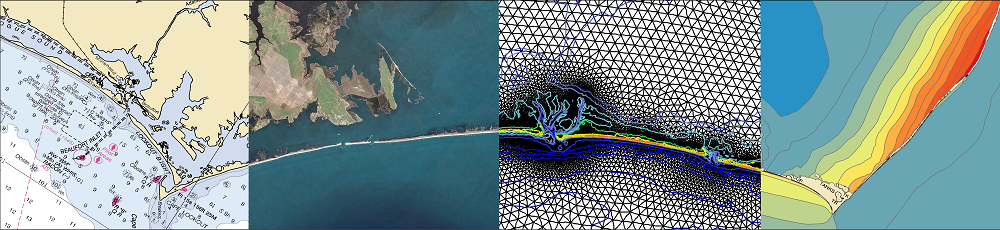
Kalpana can be used visualize and downscale ADCIRC predictions of storm surge and flooding, with documentation in a recent journal manuscript and examples in its GitHub repository. For downscaling, ADCIRC predictions can be mapped from the model resolution (e.g. 50 to 100 m or larger in coastal regions) to higher resolutions (e.g. 10 m or smaller in a DEM). The downscaled flood map is a better representation of the hazard.
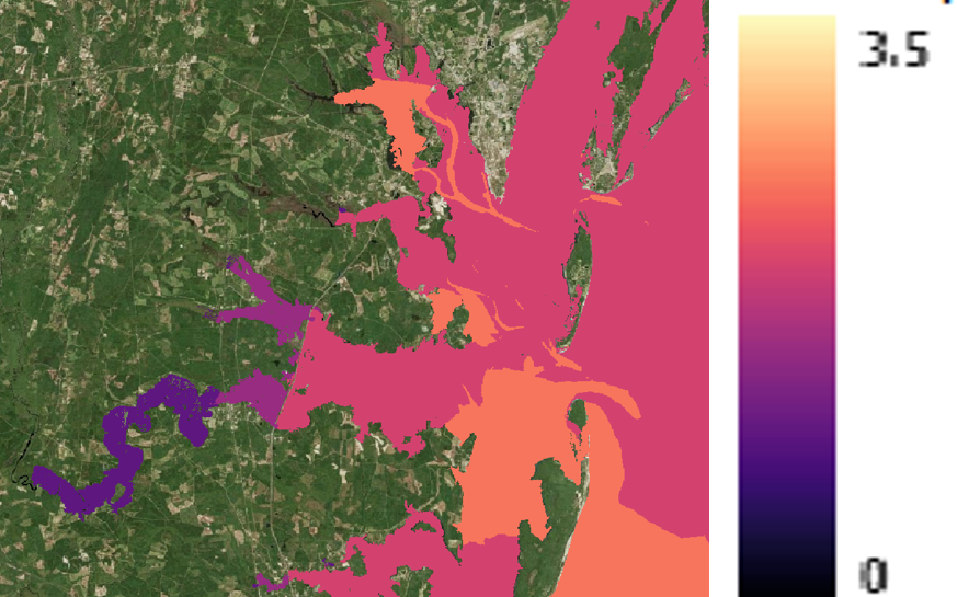
Maximum water levels along the Georgia coast due to Hurricane Matthew (2016) as visualized by Kalpana.
However, as an input for downscaling, Kalpana requires a raster DEM as a target. DEMs can be quite large, and thus it can be challenging to store and share them for other users. It is better for each user to develop their own DEM, with a specific focus to their region of interest and a specific resolution. On this page, we provide information about how to create DEMs for use with Kalpana.
Please continue reading for information on how to construct DEMs!
Downloading CUDEM Tiles
A good resource is the Continuously Updated DEM (CUDEM), which offers a database of tiles at this link. Instead of downloading the tiles for the entire U.S. coast, you can download only the tiles you need:
- Download the Tile Index (tileindex_NCEI_ninth_Topobathy_2014.zip), unzip it, and open it in your favorite GIS software. (For this examples, we will use the open-source QGIS.) To open the shapefile in QGIS: (a) open a new project, (b) go to the layer tab on the top of the screen, (c) add layer, (d) add vector layer, and (e) use the three dots to select the shape file you just downloaded.
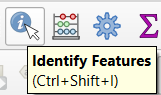 The tile index should appear as a set of rectangle polygons along the entire U.S. coast. You can query each tile by using the ‘Identify Features’ tool. With this tool, you can click on one or more rectangle polygons, and an information panel will open in the lower left of the screen. The information panel will include a link to the DEM (GeoTIFF).
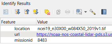 It is a good idea to also load a shapefile with the extents of your ADCIRC mesh, or at least the floodplains where you want to downscale the ADCIRC flood predictions. If you can identify your region of interest, then it will be easy to identify which tiles to download.
Merging Tiles into a Single DEM
Let’s work through an example that creates a DEM for the southernmost point of Florida.
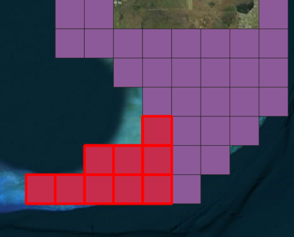 Use the ‘Identify Features’ tool to select 5-10 connected tiles in south Florida as shown. Again, depending on your region of interest, you may need more or fewer tiles to cover the floodplains. But for this example, let’s use the tiles only in the Florida Keys. After the tiles are selected, then in the information panel, use the links to download the tiles.
- After the tiles have been downloaded, they can be loaded into QGIS by (a) using the dropdown menu for ‘Raster’, (b) selecting the option for ‘Miscellaneous’, and (c) selecting the option to ‘Merge…’.
- A window will open that asks for various information and parameters, including the input layers. Click the three dots beside ‘Input layers’ and then select ‘Add File(s)’ to identify the tiles you downloaded. Then click ‘OK’.
- Return back to the original window. To allow the software to differentiate between a water level of zero versus a null value, go to ‘Assign specified ‘nodata’ value to output’ and set it as -9999. This will clean up the DEM.
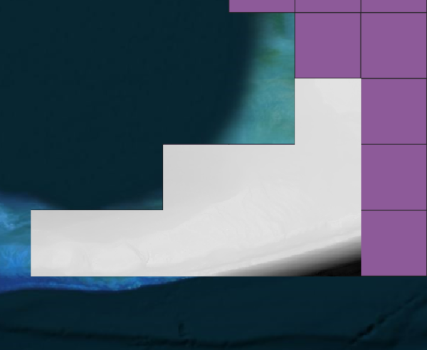 After the inputs and parameters are set, run the merging process. This may take a few minutes. When the process is finished, the DEM will be trimmed to match the shape of the tiles without the surrounding null data. Additionally, the selected tiles will change from a solid color to a topographical map of the area. It will likely be shown in grayscale (see example at right), and there may not be much color variation due to the low-lying topography.
- For the last mandatory steps, go to the Layers panel, right-click on the new merged layer, then select ‘Export’ and ‘Save As’. This will bring up an Export window with options. Click the globe symbol and enter a target projection (EPSG). In this example, we used the unique EPSG (32617) for the Southern Florida, but the choice of projection is left to the user. Kalpana can work (at least theoretically) with any projection for the raster DEM, but we find it is better to stick with projections that have horizontal units of meters (or feet). So UTM zones and similar projections are best.
- In that Export window, you can also resample the DEM to a target horizontal resolution. In this example, we change the resolution to 15 m, which should be much finer than any ADCIRC mesh. But again, the choice of resolution is left to the user. Coarser resolutions will lead to smaller DEMs and faster processing times.
- Click ‘OK’ to export the raster DEM.
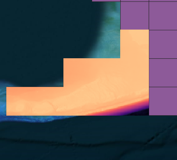 As an optional step, If you’d like to change the color gradient of the newly merged file, double-click it on the Layers panel, and switch the render type from ‘Singleband gray’ to ‘Singleband pseudocolor.’ I prefer to alter the ‘Color ramp’ because it has preset colorways that help highlight different parts of the file. This color change does not affect the DEM, but it does change how it is visualized in this session of QGIS.
You have now created your very own DEM!